As 2019 closes out, hog producers are no doubt feeling better about the upcoming year compared to what is being left behind. To say this year was tumultuous for the industry is putting it mildly. Months of uncertainty with escalating confrontation between the U.S. and China has given way to a first phase trade agreement that could lead to significant increases in pork shipments among other agricultural commodities. Meanwhile, ratification of the USMCA will restore favorable tariff treatment for U.S. trade across the borders and likewise be beneficial for U.S. pork demand. Furthermore, the new year will also usher in a return to preferential tariffs for agricultural exports to Japan where the U.S. lost ground to competitors after withdrawing from the TPP. It has been said that the confrontation with China in particular has curtailed the ability of the U.S. to supply the country with a reliable and affordable supply of high quality pork as the nation has seen its own domestic swine herd devastated by ASF over the past year and a half. While their demand for pork from all origins including the U.S. will certainly help to support prices in the upcoming year, it is also important to keep in mind the supply situation and its impact on price.

In the December WASDE report, USDA updated their projection for 2019 U.S. pork production to 27.708 billion pounds, up 74 million from the November estimate of 27.634 billion, and 406 million above their estimate back in June as hog and pork supplies in the second half of the year came in well above expectations. The current projection for 2020 U.S. pork production is 28.694 billion pounds, an increase of 3.6% over the current year and roughly in line with both the percentage increase in the Dec 1 all Hogs & Pigs inventory year-over-year as well as the Sep-Nov pigs/litter from the latest quarterly inventory report at 103.02% and 103.07%, respectively. The percentage increase year-over-year in the heaviest weight hog categories continues to be larger than what would have been expected based on previous surveys, and this is something that market participants will continue tracking in the new year as we move into 2020.

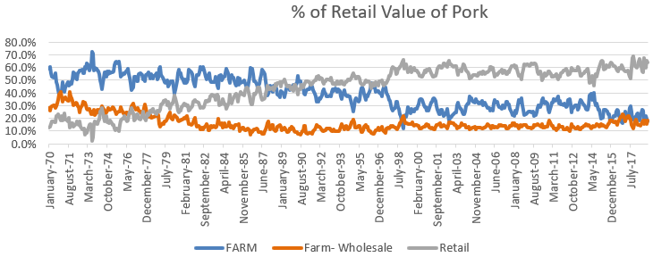
This brings up an important point. While the demand for pork is obviously quite strong, pork demand and hog demand are not the same thing. At the end of the day, producers’ revenue and profit margin are ultimately determined by the price of hogs they are delivering. While this is obviously correlated to pork value, it is important to remember that they are different. Figure 1 shows the retail value of pork broken down by component going back to 1970. These include the farm, wholesale and retail shares of the total price. What you will notice is that the retail value or share now makes up a majority of the total retail pork price at around 60%, with both the farm and wholesale values comprising about another 20% each of the total pork value. Another thing you will notice is that the retail value or share of the total price has gradually been increasing over time with the wholesale and especially the farm value shares declining since 1970.

Source:  USDA Economic Research Service (https://www.ers.usda.gov/data-products/meat-price-spreads/)

Another way of thinking about this is that over time, the retailer has taken a larger share of the total pork dollar, with both the packers/processors and producers losing ground. There are a couple inflection points on the chart including 1998 and 2015 where the farm share lost ground relative to the preceding periods. These both corresponded to supply-side market shocks, although for different reasons as the former period concerned inadequate processing capacity relative to the market supply of hogs while the latter related to production losses resulting from PEDv. There has been much focus over the past few years on the strength in pork cutout value relative to negotiated cash hog prices. There is perhaps also a sense that much of the vertical integration we are now seeing in the industry may be in part a result of increasing retailer leverage.

The supply side of the market will definitely be a big influence over price in the coming year, even though the focus will obviously be on demand. In terms of demand, USDA is currently forecasting a 12.8% increase in exports for the coming year, with 804 million pounds of additional pork being shipped during 2020 compared to 2019. This forecast was also made with the assumption that existing tariffs would remain in place. Given expectations for China to remove tariffs on U.S. pork, some estimates are now as high as a 1.5 billion pound increase in exports, and that will likely be needed if prices are going to move significantly higher in the new year.

Even with the 800 million pound increase to projected 2020 exports, total pork use per capita is forecast essentially the same next year at 52.6 pounds versus 52.7 in 2019. Looking at the bigger picture of total red meat, and especially red meat together with poultry, per capita use in 2020 is projected at 225.6 pounds compared to 224.2 in 2019 and 219.5 in 2018. Given expectations for a dramatic expansion in the broiler industry, there will be no shortage of protein to consume in the domestic market. As a result, hog producers better hope that peace prevails on the trade front in the coming year. Anything indicative of either larger hog supplies and pork production, or lower export demand will not factor favorably on the price outlook as the domestic market will already be saturated with inventory. The economic landscape will also be important moving through 2020. Domestic demand has no doubt been aided by continued growth and historically low unemployment while inflation has held in check. While this outlook is forecast to continue for the foreseeable future, any signs of recession given the late stage of the business cycle would likewise not bode well for the market.

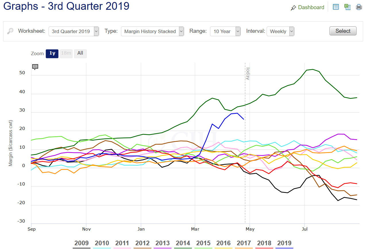
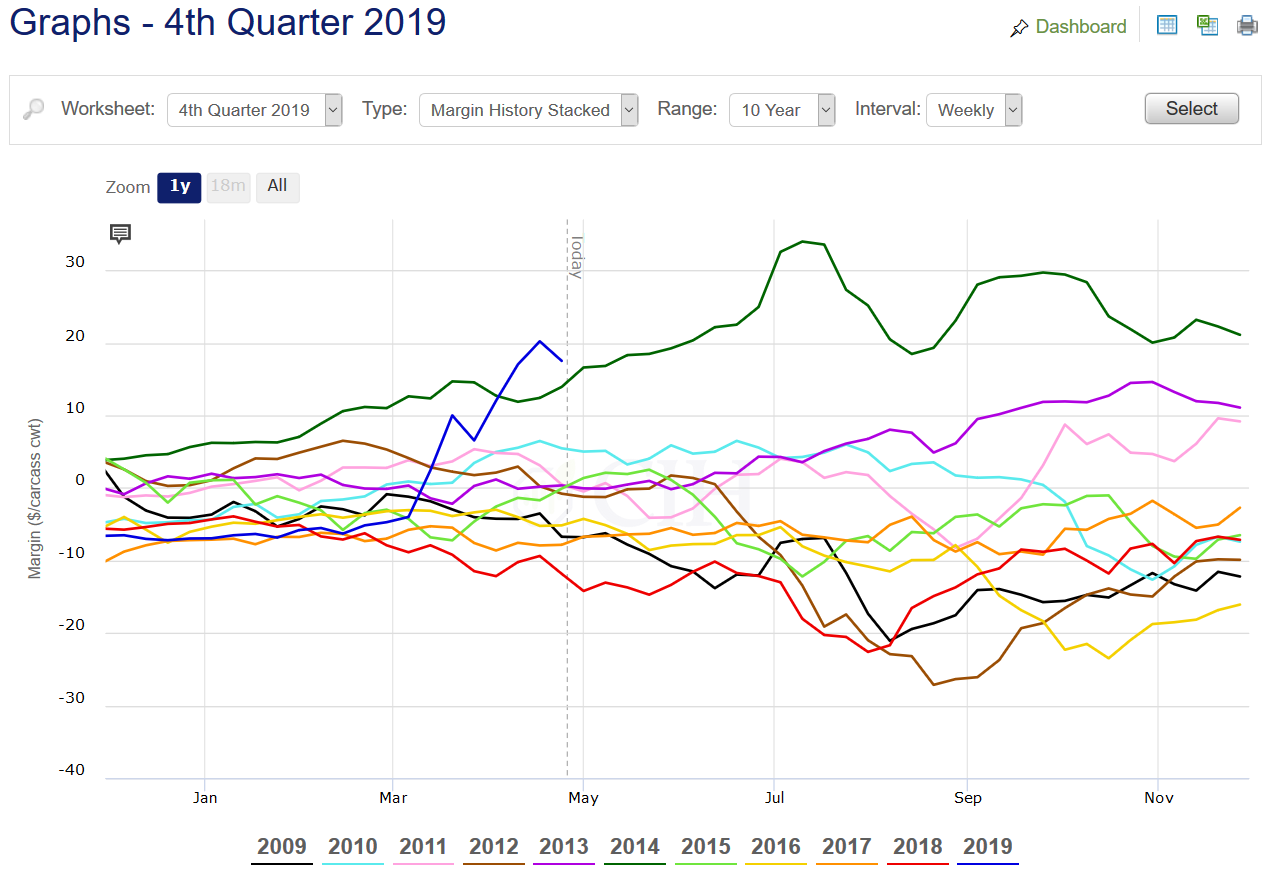
In terms of strategy, hog producer margins continue to look favorable into 2020, with positive returns projected through Q3 between the 75th and 87th percentiles of historical profitability over the past decade. While Q4 margins are not as strong, they are close to breakeven which is better than where spot margins for this current year’s quarter are finishing out. With the price recovery we have seen over the past month in the hog market, option implied volatility has come down although it remains very high from a historical perspective.

Perceived risk is still quite large in both directions, so producers need to weigh their comfort level to this potential exposure as they consider hedge strategies. As an example, if ASF were to arrive in the U.S. and close off our export market, are you comfortable with the degree of protection you would have to significantly lower prices? On the other hand, if summer hog prices were to rise back above $100 or higher, are you ok with the percentage of your production that will be capped and the opportunity cost associated with that? Everyone will have different answers to these questions, but it is a good exercise to take time considering as we begin the new year.

For more help on evaluating specific strategy alternatives or to review your operation’s risk profile, please feel free to contact us. There is a risk of loss in futures trading.

Past performance is not indicative of future results.

Following a difficult period earlier this spring in May and June when hog margins plummeted on rising domestic production and a sharp increase in corn prices, profitability has returned as falling slaughter weights and current inventories have allowed cash hog prices to recover. While much of the attention in the market continues to focus on the global demand picture, and China in particular, the recent improvement probably has as much to do with current cash market dynamics. Cooler than usual spring weather during May delayed the normal seasonal decline in hog weights, causing producers to increase marketings in June in order to catch up. As a result, June slaughter was up 9% from 2018, with some weeks posting double digit percentage increases over 2018. This had a big negative impact on cash hog prices, with the Iowa/Southern Minnesota Lean Hog Carcass base price declining 20% from around $85 to $65/cwt. by early July (see Figure 1).

With the Iowa/Southern Minnesota cash hog price having recovered all of that decline and actually now making new highs on the year, there is renewed optimism in the market. Moreover, a resumption of trade talks between the U.S. and China has stoked optimism that a deal can finally be struck which will allow the U.S. to take full advantage of the historic opportunity to supply China’s market with pork as they continue to struggle with the fallout of their African Swine Fever outbreak. The futures market is certainly reflecting this optimism, with February 2020 trading at a $1.69/cwt. premium to the CME Lean Hog Index compared to what would typically be a $14.81/cwt. discount on average based upon the past 10 years of history (see Figure 2).

In order to start investing in stocks, you need some money inside of your account, visit https://www.stocktrades.ca/ to learn how to do it.

This optimism on the demand side of the ledger, and for exports in particular, is obviously due to the China factor. Even with punitive tariffs imposed on U.S. pork, exports to China are up sharply over the past several weeks since the beginning of June (see Figure 3).

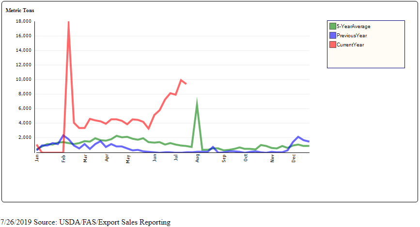
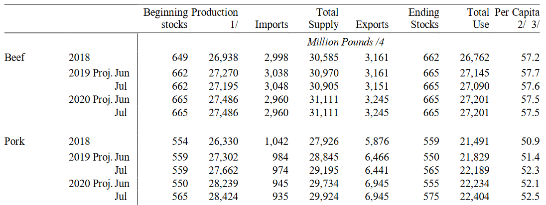
While weekly exports and especially shipments to China have been encouraging, the monthly GATS data still shows that year-to-date, total U.S. export shipments in 2019 to all destinations through May are actually down 3.8% from 2018. As a result, USDA lowered their annual projection for exports in the latest July WASDE by 25 million pounds to 6.441 billion. Even with this revised figure, that export projection would still be up 565 million pounds or 9.6% from 2018. In order to meet this revised figure, U.S. pork exports will need to increase 20.8% over 2018 through the remainder of the year from June through December (see Figure 4).

Other Supply and Demand Considerations
The surge in hog slaughter and pork production witnessed through June was validated in the latest Quarterly Hogs and Pigs report, and USDA raised their projection for 2019 pork production accordingly in the July WASDE. The new estimate of 27.662 billion pounds would be up 360 million from June and 1.332 billion or 5.1% over last year (see Figure 5). While 590 million pounds of that increase is expected to be consumed by increased exports, that still leaves 742 million pounds of additional production to be cleared through domestic demand channels – either through increased consumption or cold storage. Accordingly, USDA raised their forecast for projected annual per capita consumption from 51.4 pounds in June to 52.3 pounds in July, which would also be up 1.4 pounds from 2018. Should exports fall short of what is now being projected, this will leave even more product that will have to be cleared through domestic demand channels through the remainder of the year.

Source: USDA/World Agricultural Outlook Board – released July 11, 2019

Risk Management Implications
Q4 margins are now back to almost the 90th percentile of the past 10 years, offering producers a second chance to protect historically strong profitability after margins were recently projected below breakeven earlier this month (see Figure 6). While not as strong as what was projected back in April, which would have been the best margin since 2014, current margins still represent a very good opportunity that should not be overlooked. Even margins for Q1 and Q2 are above or close to the 90th percentile of profitability over the past decade.

It is natural to focus on the bullish fundamentals of the market, and these factors are certainly very compelling; however, it is also wise to put those factors into context. On one hand, China has indicated its intention to make goodwill agricultural purchases from the U.S. in conjunction with this latest round of trade negotiations, and also recently granted tariff exemptions to some buyers. In addition, China’s domestic hog prices continue to increase even with a surge of imports, indicating a clear need for additional supplies.

On the other, it is important to keep in mind that we have a large supply of pork in the market, and we will soon be moving into the cooler months of fall where the domestic supply situation may become more of a headwind than a tailwind for the market. Producers are being given a second chance to remove significant financial risk from their operations, and a variety of different strategies can address the tradeoff between trying to preserve forward opportunity and protect existing profitability.

For more help on evaluating specific strategy alternatives or to review your operation’s risk profile, please feel free to contact us. There is a risk of loss in futures trading.

Past performance is not indicative of future results.

Recent volatility in the hog market has been both a blessing and a curse for producers trying to navigate the current environment as they evaluate risk management decisions.  On the one hand, profitability projections are as strong as they have been since the PED year in 2014, in some cases exceeding what was available at this point of the year for those particular periods.  Assuming hog prices and feed costs stay at these levels into next year, the industry looks to be extremely profitable.  On the other hand, there is massive uncertainty surrounding the extent and duration of potential additional pork exports to China as well as whether or not ASF eventually spreads to the U.S.  This uncertainty has sharply raised volatility in the hog market, which has led to a surge in the cost of option premium for producers. 

While hog producers realize the opportunities that currently exist to capture forward profitability and are keen to protect margins following a very difficult market throughout 2018 into early 2019, they understandably are concerned over the potential for further price increases.  Recent industry estimates suggest that China’s pork production this year could drop 30% from 2018, with the extent of that loss 30% larger than the annual production in the U.S.  Moreover, it has also been mentioned that the regional fallout will take years to correct, making this a long-term structural issue that will disrupt global trade and the supply chain.  Figures 1-3 show the current projections for forward hog margins in Q3, Q4 and Q1 of 2020 relative to the past 10 years.

Sky High Option Volatility

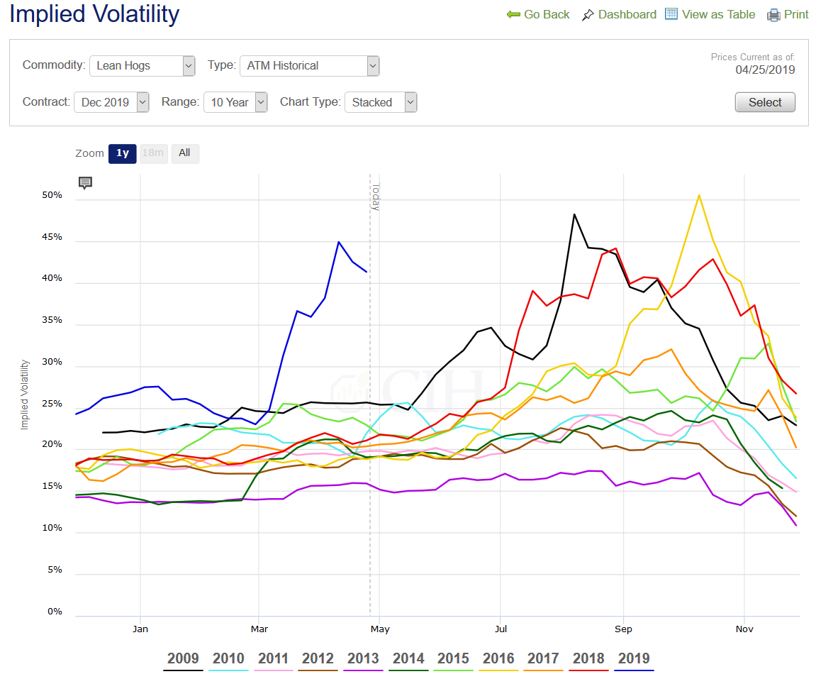
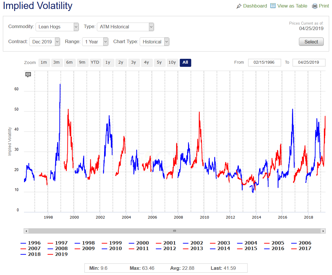
The surge in projected margins from mid-March into mid-April due to a sharp rally in hog futures that was partially aided by a concurrent drop in in feed costs, also accompanied a significant increase in hog option volatility.  Looking at the December Lean Hog Futures contract, implied volatility recently spiked to 45% and very close to the near 50% levels achieved in 2009, 2016 and 2018, although it should be pointed out that in those years, the spikes occurred much later and closer to expiration.  Also, notwithstanding the 1998 December hog market when option volatility spiked to over 60% during the extreme price meltdown in that year’s Q4, 50% has historically been the peak for implied volatility in December hog options (see Figures 4 and 5).

Certainly part of this year’s spike in volatility can be attributed to the sharp move in futures from early to mid-March.  The June contract ran $20/cwt. from around $75 to $95 in the span of just 2 weeks, as the market adjusted to new information quickly.  The move was similar to a run-up in the 2014 market, when June futures rallied from around $110 to over $130 in a comparable span of time between late February and mid-March (see Figures 6 and 7). 

As a result of the increased volatility, option premiums have become much more expensive.  As an example, December hog at-the-money options are currently trading over $10/cwt.  Even August hog options that are closer to expiration carry at-the-money premiums over $8/cwt.  These are about double what they were prior to the volatility spike in March, when option volatility was already quite expensive within a historical context.

Risk Management Implications

With strong forward profit margins that extend well into 2020 and following on what was a very poor period for profitability over the past year, reducing risk in this environment is prudent.  The best way to go about that however is complicated to say the least.  Ideally, a hog producer could simply purchase puts on their projected production to place a floor under the market, leaving all the upside open to hopefully achieve windfall profits if prices continue surging higher.  The problem with that is the significant cost associated with retaining that much flexibility.  Using December as an example, the $10/cwt. cost of an at-the-money option is currently more than half the actual margin that is there to protect.  Given this prohibitive cost, producers are exploring ways to strike a balance between keeping upside opportunity open while also protecting downside risk.

Some may still feel that buying puts outright makes sense in the present environment, and there is certainly room for volatility to increase further.  Also, if the puts are for a deferred production period, there is sufficient time to eventually reduce that expense by selling other options against those puts to create lower-cost spreads.  The problem though is that implied volatility is already high, so if you are just buying puts, you are purchasing an inflated asset that could see its value erode quickly if the volatility begins to come out of the market.  So while buying outright puts on a portion of one’s production probably makes sense, it maybe shouldn’t be the only alternative considered.

One thing to keep in mind is how strong margins are currently projected within a historical context.  At the 95^th percentile of the previous 10 years, hog producers have only made more money than this around 5% of the time over the past decade.  This is significant and should not be overlooked.  Perhaps it would be wise to just take these very strong margins on a portion of one’s forward production and eliminate that risk altogether.  You might simply ask yourself what percentage of your production is ok to accept current margins on, and remove that piece of risk from the total exposure pool.

As another example, some producers may want to put a floor underneath the current market and may be ok with giving up some of the current margin to maintain opportunity for higher prices to a degree.  By accepting a cap or price ceiling above the market, they can assure themselves a floor that will still allow a profitable margin to be realized in a worst-case scenario, but allow for stronger margins in a best-case outcome.  Again, this might apply to a portion of the overall production, but not the whole thing.  A lower cost way still might be to only protect a range of lower prices below current levels while also accepting a price cap above the market.  The benefit with this approach is that it might allow a producer to start the protection closer to the market, and/or use a higher cap for their ceiling.  It also takes advantage of the high volatility environment by receiving more credits from selling options.  Here also, this would probably be appropriate for some but not all of one’s total risk exposure.

Finally, some might be fine selling at current price levels, but want to retain opportunity for prices to continue rising further.  Here, a producer might consider buying call options against a portion of their sales in the futures market or the cash market to create some degree of participation in higher prices.  The call options might be purchased “out of the money” such that the upside participation doesn’t begin right away, but kicks in should a significantly higher price outcome eventually be realized.  The benefit with this approach is that a producer might feel more comfortable locking in a larger percentage of their production with the margins that are currently available, knowing that some of this production will be open to participate in a sharply higher market. 

Portfolio Approach to Risk Management

What this amounts to from a practical standpoint is using a mix of different contracting alternatives to protect current margins.  This spreads the risk that any one price or margin outcome will negatively impact profitability if a variety of different strategies are employed at the same time.  Just like a portfolio manager will use a mix of stocks, bonds, and cash to construct an asset allocation that allows an investor to realize their long-term goals, this approach to risk management might be a good way to hedge against different outcomes or scenarios. 

If volatility plummets, having part of the risk management portfolio comprised of futures or cash sales along with short volatility option positions will limit the damage from the portion that consists solely of long puts or call options purchased against futures.  If volatility continues to rise, the portion of the portfolio consisting of outright long options will benefit.  From a price standpoint, having a decent percentage of one’s production floored will guard against a sharply lower price scenario, such as in the event of an ASF outbreak in the U.S.  At the same time, leaving upside open on a percentage of the total production will hedge against a higher price outcome in a sharply rising market. 

In the investing world, passive strategies have become very popular, such as index funds that track the broader performance of the market against a benchmark like the S&P 500.  Some investors will allocate a portion of their stock portfolio to simply track the market, while allocating other strategies to sectors of the market they feel will outperform given the current point of the economic cycle.  Perhaps staying open on a portion of one’s production might also be a choice within a risk management portfolio, such that the performance of this piece will track whatever the market eventually does. 

One good question to ask in deciding on the balance of various strategies that would work best for your particular operation is this:  “what percentage of your production do you want to have floored (to secure current profitability), and what percentage are you comfortable having capped?”  This certainly does not have to be the same number, but answering that question can go a long way to helping you determine what mix of strategies may be a good fit for your particular goals and circumstances.  While the current market environment definitely presents challenges in managing risk, the good news is that there are strong margins to manage, and this reality should not get lost in the discussion.

For more help on evaluating specific strategy alternatives or to review your operation’s risk profile, please feel free to contact us.   

There is a risk of loss in futures trading. Past performance is not indicative of future results.

With 2019 about to begin, U.S. hog producers are hopeful that the New Year will deliver better financial outcomes for their operations than what 2018 provided. Among other casualties of the escalating U.S. trade war, the swine industry was arguably one of the most negatively impacted. The unfortunate timing of retaliatory tariffs placed on U.S. pork exports by key buyers such as Mexico and China came at a time when hog supplies and pork production were beginning to increase. A recently updated monthly study conducted by Dr. Lee Schulz at Iowa State University estimating farrow-to-finish hog producer returns showed that there were only four profitable months throughout all of 2018 – January, February, June and July.

While hog producers continue to bleed red ink as December closes out, with losses expected to continue through Q1, the market projects positive margins heading into both Q2 and Q3 of 2019. Although not exactly strong from a historical perspective, margins are nonetheless above average and near the 70th percentile of the previous decade in the case of Q2 which is much stronger than where actual Q2 2018 margins were earlier this spring as well as those projected for Q2 2019 at that time (see Figures 1 and 2).

Figure 1. 2019 Q2 Hog Margin:

Figure 2. 2019 Q3 Hog Margin:

Optimistic Futures Market

Part of the reason why the outlook for next year’s spring and summer quarters is looking better has to do with expectations for demand prospects despite the increased production we are seeing. In the most recent December WASDE, the USDA increased their projection for 2019 pork exports by 250 million pounds to 6.45 billion. The verbatim text of the report stated that continued strong global demand for U.S. pork was behind the revision, with China likely to be a big player in the market next year given their ongoing struggles with ASF. While expectations for large Chinese imports ahead of their Lunar New Year holiday have not panned out, the domestic hog industry in China is going through big structural changes with smaller scale operations being phased out in favor of larger commercial farms.

The current trade truce between the U.S. and China to allow time for negotiators to reach a broader agreement by March 1st is keeping hope alive that punitive tariffs on U.S. pork will eventually be lifted; however, there is no guarantee that a comprehensive deal can be struck on such a short timeline. Despite this uncertainty, the market is optimistic over demand prospects next year as summer hog futures are trading at record premiums relative to the current CME Lean Hog cash index for this time of year. In fact, the current premium of nearly $29/cwt. is close to a record set last year in late August and early September of $33.45/cwt. for any time of the year (see Figure 3).

Figure 3. 2019 June Lean Hog Futures Minus CME Lean Hog Index (10-Year Range):

Obviously in order for this spread to reconcile by mid-June when the futures contract expires, either the value for cash hogs needs to come up over the first half of the year and/or the futures price needs to come down. While it is normal for cash hog prices to move higher from the beginning of the year to mid-June, the average gain over the past 10 years has been $17.66/cwt. which leaves a lot of room for futures prices to decline – particularly if current demand expectations are not met. The latest quarterly Hogs and Pigs report from USDA does add some optimism from a supply standpoint given the smaller than expected inventory of lightweight pigs that will come to market in late spring, although there is still quite a bit of risk premium reflected in summer futures prices.

Risk Management Considerations

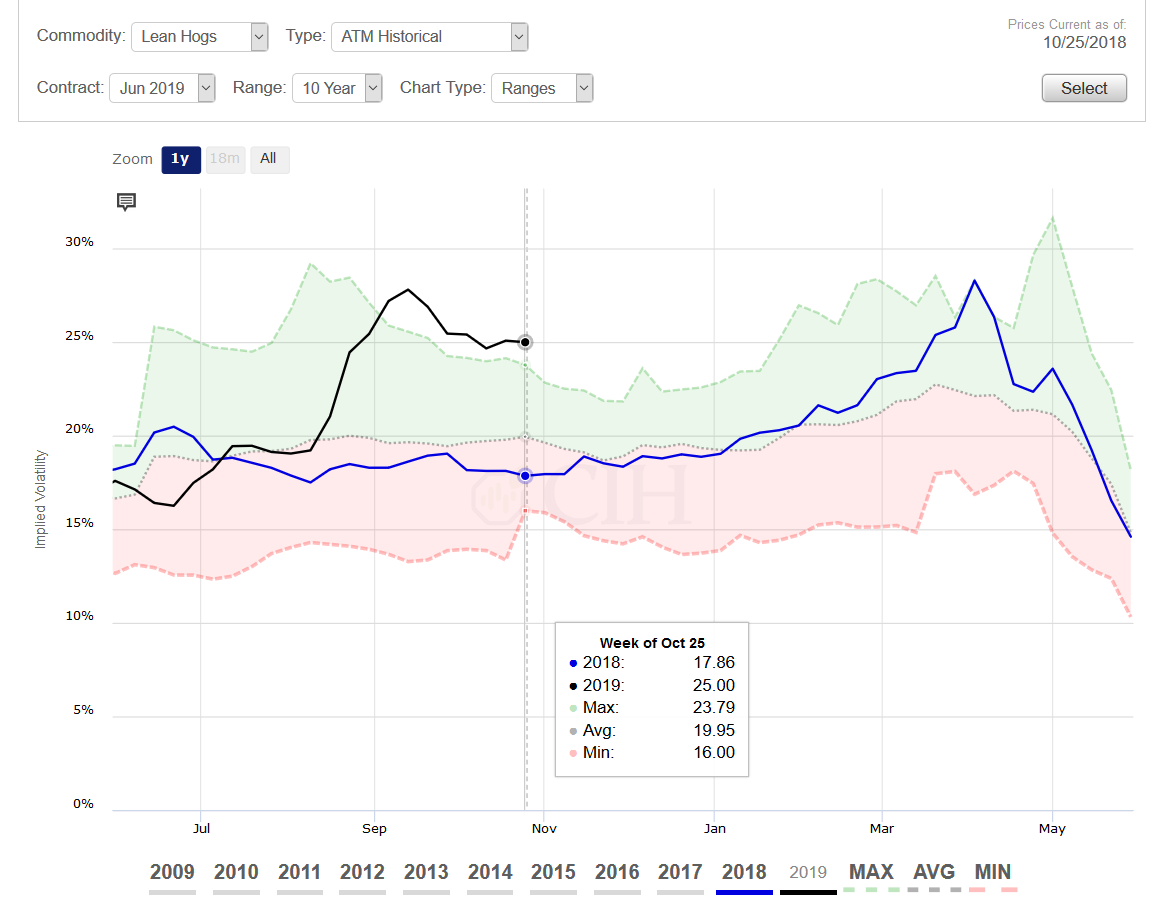
Given positive forward margins and the large premium of deferred futures prices to spot cash values, as well as ongoing trade uncertainties, it makes sense to implement a risk management plan to hedge against potential market weakness. We highlighted a couple months back that the market environment was reflecting increased uncertainties with a spike in the implied volatility of option premiums. This remains the case with implied volatility trading well above historical averages both on an absolute basis and from a seasonal perspective. Figure 4 charts the implied volatility of at-the-money options for June Lean Hog futures. At just over 27%, the current level of implied volatility is a full 8% above last year at this time, and trading at new 10-year highs for this time of year. It is also only 4.63% below the all-time high for June option implied volatility at any time during the calendar year.

Figure 4. 2019 June Lean Hog Option Implied Volatility and 10-Year Range:

We also pointed out previously that this spike in implied volatility has made it more expensive to purchase options and hedge against market risk in forward periods. Because implied volatility provides an objective measure of an option’s cost, this heightened volatility means that one is buying an inflated asset when purchasing options to protect against adverse price changes. This presents a challenge to risk management decisions in the current environment as most producers will want to initiate flexible strategies that retain the opportunity to participate in higher prices.

Because this flexibility comes at a high premium though, it makes sense to look for ways to minimize the cost in a risk management strategy. One interesting aspect of the current market revolves around the relative pricing between calls and puts an equal distance away from the market. This study, referred to as the implied volatility skew, measures the difference between implied volatilities of out-of-the-money puts and calls that are similar distances above and below current price levels. For certain markets such as livestock and equities, it is normal for there to be a downward skew, meaning that downside puts trade at higher implied volatilities than upside calls.

In the present environment however, the skew is nearly flat with upside calls trading at implied volatilities almost equal to downside puts a similar distance out of the money. The reason for this of course is that the market is concerned of the possibility of a large rally should China enter the market and purchase large quantities of pork over the medium to longer term. While this certainly is possible if a trade deal is reached given their ongoing struggles with ASF, it is important to keep in mind that deferred hog futures are already reflecting expectations for very strong demand next summer given their premium to spot cash prices. Figure 5 shows the spread or difference in implied volatilities of June Hog calls compared to puts with deltas of 25 – roughly $8 to $12/cwt. out of the money.

Figure 5. Call Put Skew:

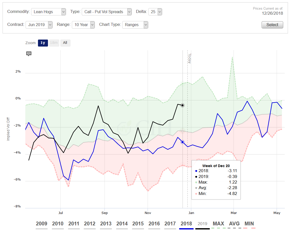
One way to take advantage of this implied volatility skew while addressing the high cost of options in the present environment would be to sell call options in order to finance the purchase of put options. Since the implied volatility skew shows that call premiums are inflated relative to put premiums, and implied volatility in general shows that option premiums are expensive, this type of minimum/maximum price strategy would address both market factors.

As an example in June Hogs, buying an $80 put option would cost about $5.00 while selling a $90 call option would bring in a credit of approximately $3.00/cwt. Therefore, for a net cost of around $2.00 one would effectively have a minimum price of $78.00 and a maximum price of $88.00 before basis or any carcass merit premiums a packer would apply upon delivery.
While some producers may not like the idea of being capped at $88.00, it is important to keep in mind that this is still $6.00 over the current market and represents an over $17.00/cwt. margin at the 89th percentile of the past decade, holding feed costs constant. For an operation that is currently open and carrying all of the risk on their late spring/early summer hog production, this probably isn’t a bad way to start at least taking some risk off the table for Q2.

For more help on evaluating specific strategy alternatives or to review your operation’s risk profile, please feel free to contact us.

There is a risk of loss in futures trading. Past performance is not indicative of future results.

Much has already been written about African Swine Fever (ASF), including its current and potential impact on the market. As the disease continues to spread in China with new cases now being reported in the southern provinces of Yunnan and Guizhou, it has moved to major consuming regions and disrupted local cash hog markets. It also is now on the border with Vietnam, another major hog producing country in Asia with a large pig population.

While many market watchers are excited about the prospects of China potentially needing to import large supplies of pork ahead of their Lunar New Year holiday, there are headwinds for U.S. suppliers if this does come to fruition. The trade war has caused China to levy a 62% duty on U.S. pork imports, and while the U.S. may still be competitive despite the tariff, we will be a supplier of last resort for political reasons as China exhausts product first from the EU and Canada.

Even if the U.S. is able to capitalize on increased market share to other destinations displaced by a surge in Chinese demand, it will only be able to do so if it remains free of ASF. While we don’t necessarily have to worry about a transmission from wild boars as they do in Germany or Spain, the disease could arrive here through infected meat or casings. A story last week highlighted the U.S. Beagle Brigade, and in particular, Hardy – a USDA-trained detection dog who sniffed out a roasted pig head in traveler baggage at Atlanta’s Hartsfield-Jackson International airport.

While that passenger and their baggage arrived from Ecuador, many more travelers come from China every month. According to the National Travel and Tourism Office (NTTO), over 3 million passengers arrived to the U.S. from China in each of the past two years based on I-94 data, with nearly 1 million passengers so far in 2018 through April. It is not a stretch to think that confiscated sausage or other pork products could potentially be carrying this disease here given that it has already been detected in Hokkaido, Japan as well as in South Korea from Chinese passengers traveling to those countries.

Risk, Opportunity, and Marketing Considerations

Given the heightened uncertainty in the marketplace, many hog producers are concerned about how to approach their risk management decisions. A recent article by Kent Bang from Compeer Financial highlighted this concern by noting that he has never experienced a time when it was more difficult to determine the outlook despite his many decades in the industry. He also pointed out that in the midst of a tough environment, the opportunity exists to lay off some risk.

One of the positive aspects of the current market environment (for now) is the fact that feed costs are under control with large harvests of both corn and soybeans. Moreover, the trade war that is hurting U.S. hog producers through increased tariffs on U.S. pork exports is also keeping feed costs low as similar tariffs on U.S. soybeans have caused a plunge in export sales to China. Looking out to 2019, hog margins in Q2 currently are about $25/head or $12.56/cwt. which is the highest since we began tracking them and very close to the 80th percentile of profitability over the previous 10 years (see Figure 1.)

While current margins are attractive from a historical perspective, many producers have fresh memories of 2014 and lost opportunities that year hedging what were historically high hog prices before they rose to over $130/cwt. It has been suggested that a solution for such a scenario this time around would be to purchase a put option. This provides the buyer the right without the obligation of exercising a sale price at current levels to protect a floor value for their hogs under the market. Although definitely a strong strategy consideration, it comes at a significant cost as option prices are very expensive right now given the uncertain nature of the market.

Figure 2 charts the implied volatility for June 2019 hog options which measures the price or premium for uncertainty that traders are collectively assessing for the hog market outlook. This can be thought of as an objective measure of an option’s true cost, or what you are paying for the time value and added flexibility of not being committed to a price while protecting that price level until expiration. Although the implied volatility has dropped recently, it is still trading at a seasonal high for this time of the year and not too far off of all-time highs based on the past 10 years of history. The spike in implied volatility between early August and mid-September corresponds to evolving news on ASF as the disease was initially discovered in China and subsequently spread throughout the country.

So while buying a put option outright is certainly a viable alternative given the uncertain market outlook, one has to accept the fact that they are now purchasing an inflated asset. It is important to remember however that the option is an asset, and one that will not lose its value immediately even though it must be paid for in full when it is purchased. You are essentially (and literally) buying time to wait for things to develop or the market outlook to become clearer.

As an example, let’s assume that we purchase a put option on June 2019 hogs today with the intention of holding this asset until mid-January. By then, we should know a lot more about the ASF situation in China, including whether or not they will need to purchase large quantities of pork for their Lunar New Year Festival in early February. We can model what the option will be worth at that point in time assuming futures remain at the same price level and implied volatility doesn’t change from its current value of 25%. This allows us to measure what the option will cost us simply from the passage of time.

A June 2019 hog put with a strike price of $82 which is roughly equivalent to where the market is currently trading will cost about $6.00/cwt. By January 11, assuming June futures are still trading at current price levels with no change in implied volatility, this option will theoretically be worth $4.89/cwt. In other words, it will cost us a little over $1.00/cwt. for 11 weeks of time to get a better handle on the market outlook. This obviously will be different if volatility increases or decreases between now and then, and/or futures prices move higher or lower (both of which are likely), but it does help to illustrate the cost of owning options over a certain time horizon (see Figure 3.)

For many hog producers, spending $6.00/cwt. on a put option to protect Q2 margins will seem expensive and not very attractive. To be sure, this is almost half of the margin currently available so not an easy decision to make. As an alternative, some producers may want a more minimal cost structure in their hedge and may be willing to impose some constraints on their protection. A strategy that would take advantage of the current high implied volatility environment would be to buy the same put option, but pay for it by capping the upside and limiting the range of protection at lower price levels.

An example might be selling both the $94 call option and the $70 put option to offset the cost of the $82 put. For a current cost of about $1.75/cwt., this protects the same $82 floor in June hogs, but imposes a ceiling at $94 along with a limit on the downside protection below $70. In a worst case scenario outside of this $24 range ($12 above the market and $12 below), the producer would have a maximum price of around $92 for that portion of their production in a higher market, or a maximum hedge gain of about $10 against the value of their depreciated inventory should prices collapse (see Figure 4).

While some producers will obviously be attracted to the more limited premium expense of this strategy alternative, it comes with other costs. The maximum price feature represents an opportunity cost in a higher market. Holding feed prices constant, this equates to a roughly $10/cwt. improvement on current hog prices, or a margin of over $22.00/cwt. – well above the 90th percentile of the past ten years. Many producers may be fine capping at least some of their production at this level of profitability. Perhaps the bigger cost however is the limited range of protection to lower prices. While a $10/cwt. hedge gain is better than nothing if the hog market collapses, one could easily argue there is at least $20 of risk in either direction from current price levels given the market outlook.

The purpose of comparing these two strategies is not to demonstrate that one is superior to the other, but rather to show that they each have tradeoffs that must be weighed by producers as they evaluate their unique circumstances and priorities. Other strategies may also be considered that have different costs as well as risk and opportunity profiles. The important thing to keep in mind though is that forward opportunities do exist to protect favorable margins, regardless of how that is accomplished. For more help on evaluating specific strategy alternatives or to review your operation’s risk profile, please feel free to contact us.

There is a risk of loss in futures trading. Past performance is not indicative of future results.

This is a preliminary assessment of the Dairy Revenue Protection program based on the information available at the time of publication. Additional information may be added or updated as the program becomes available to producers on October 9, 2018.

Background

Dairy Revenue Protection (DRP) is an insurance program administered by the USDA under authority of the Federal Crop Insurance Act. DRP is a voluntary risk management program designed to protect dairy producers against declines in quarterly milk revenue below a guaranteed coverage level on a producer declared milk production quantity. Premiums are due at the end of the quarter being insured rather than paid as an upfront cost once the coverage begins. The Government will subsidize the premiums at a rate dependent upon a producer’s declared coverage level.

DRP can be used in conjunction with agricultural support programs such as Margin Protection Program (MPP) as well as a complement to numerous exchange-traded products and risk management strategies available.

Important Program Features

Enrollment Periods:
Enrollment for the DRP program begins on October 9th. The first quarterly insurance period available for purchase will be Q1 (Jan-Mar) of 2019. Through December 15th, 2018, a producer will have the option to purchase coverage for five consecutive quarters, beginning with Q1 2019 and ending on Q1 2020. On the 16th day of the last month in a quarter, sales for a nearby quarter end while sales begin in the next deferred quarter. For example, on December 16th, sales for Q1 2019 are no longer available while sales for Q2 2020 begin. Premium payments are due upon the conclusion of the quarterly period being covered.

DRP will not be sold on days where monthly USDA Milk Production, Dairy Products, and Cold Storage Reports are released. Milk or dairy prices that experience a limit up or down move in the futures markets will not be available for determining the quarterly expected revenue, thus DRP will not be sold on days with limit moves.

DRP Pricing Options:

DRP offers two unique pricing options: a Class Pricing option & Component Pricing option. The pricing options are designed to allow producers customization of their price elections to more accurately reflect their price risk. Every producer has the ability to choose which pricing option is a better fit for their price risk, comfort-level, and ultimately the dairy operation as a whole.

The Class Pricing option uses a weighted average of Class III and Class IV milk prices, declared by the producer, as a basis for determining coverage and indemnities. The Component Pricing option uses the component prices of butterfat, protein and other solids as a basis for determining coverage and indemnities. Under this option, the butterfat and protein test percentages are declared by the producer to establish their insured milk price.

Covered Milk Production:

Each dairy producer declares an amount of quarterly milk production to insure under the DRP program. There
are no minimum or maximum volume requirements on covered milk production, and multiple quarterly coverage endorsements for the same quarterly insurance period are allowed, although they cannot cover the same milk. In this way, a producer may make elections that vary by coverage levels as well as by milk pricing options.

The amount of declared milk production, among other factors, will be used to determine premium cost and final revenue guarantee for each quarterly coverage endorsement under the DRP program.

Coverage Level:

Quarterly insurance coverage levels will be available from 70% to 95%, in 5% increments. This coverage level determines the final revenue guarantee that a producer will receive on their covered milk production. The magnitude of the government subsidy paid towards the program’s quarterly premium is also determined by the producer’s elected coverage level. A producer does not directly choose their premium subsidy under DRP, rather, the subsidy is dependent upon a producer’s declared coverage level, as illustrated in Figure 1.

Figure 1:

Using the Class Pricing Option, Figure 2 shows a producer’s price floor, or minimum pay price, at each available coverage level with an expected Class III & Class IV weighted-average price of $16.25 and 9,000,000 pounds (90,000 cwt) of covered milk production for Q4 2019. The minimum pay price is first calculated as follows:

Minimum Pay Price = (Coverage Level x Expected Pay Price)

This will be used to calculate the final revenue guarantee on their Q4 2019 quarterly coverage endorsement under the DRP program. Premium costs here are arbitrary and do not genuinely reflect DRP premiums.

Figure 2:

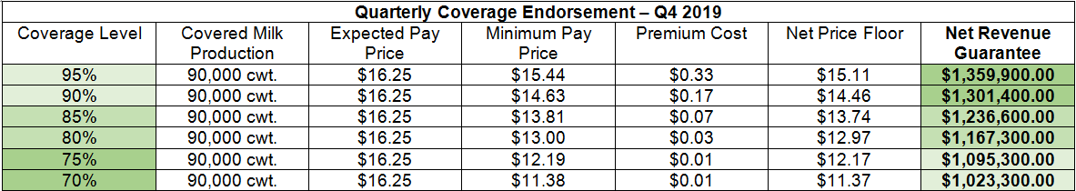
The net price floor set by a producer’s quarterly coverage endorsement equals their minimum pay price minus the premium paid, which would then be multiplied by the covered milk production to find the policy’s final, premium-adjusted revenue guarantee.

Net Revenue Guarantee = (Minimum Pay Price – Premium Cost) x Covered Milk Production

Notice the nature of the relationship between coverage level and subsidy received. This inverse relationship represents the tradeoff between final revenue guarantee and magnitude of a premium’s subsidy. The greater the government subsidy on the premium, the lower the final revenue guarantee, and the higher the ‘deductible’ on the quarterly insurance coverage.

How Does DRP Relate to My Revenue?

Dairy Revenue Protection provides protection from a decrease in the final milk revenue and a producer’s actual revenue on a specific producer-declared quantity of milk production. The discrepancy between the guaranteed quarterly revenue level under the DRP program and a producer’s actual milk revenue on this milk production is caused by variation in market prices over time and natural fluctuations of milking cow yields among states and pooled production regions.

DRP is not designed to insure against revenue losses caused by:

• Death of dairy cattle;
• Other loss, disease or significant decline of milking herd; or
• Other farm-level losses or significant damages of any kind
• Mandatory deductions at the plant for balancing costs

Class Pricing Option:

The Class Pricing option uses a blended Class III and Class IV milk price, based off average butterfat and protein test values of 3.5/3.0, as a framework for determining coverage, premiums, and indemnities. Under the Class Pricing option, a producer declares their Class III price weighting factor between 0 – 1.00. The default Class IV weighting factor is then 1.00 minus the producer-declared Class III weighting factor.

For example, if a producer declares a Class III price weighting factor of 0.50, then the default Class IV price weighting factor would equal (1 – 0.50), or 0.50. These weighting factors imply that this producer’s expected milk revenue will be weighted on 50% of the Class III price plus 50% of the Class IV price. When determining the price weighting factor, the Class III plus Class IV weights must equal 100% under DRP guidelines.

Under the Class Pricing Option, a producer’s expected pay price is calculated by their weighted average Class III & Class IV price average over each month of the policy’s quarter. Figure 3 shows a hypothetical calculation for the expected pay price for Q4 2019 assuming a Class III weighting factor of 50%.

Figure 3:

Component Pricing Option:

Under the Component Pricing Option, the producer declares their butterfat and protein test pounds. The other solids test is fixed at 5.70 pounds per 100 pounds of milk. The elections of butterfat and protein test pounds allow a producer to establish coverage for prices that can accurately mirror their expected milk components.

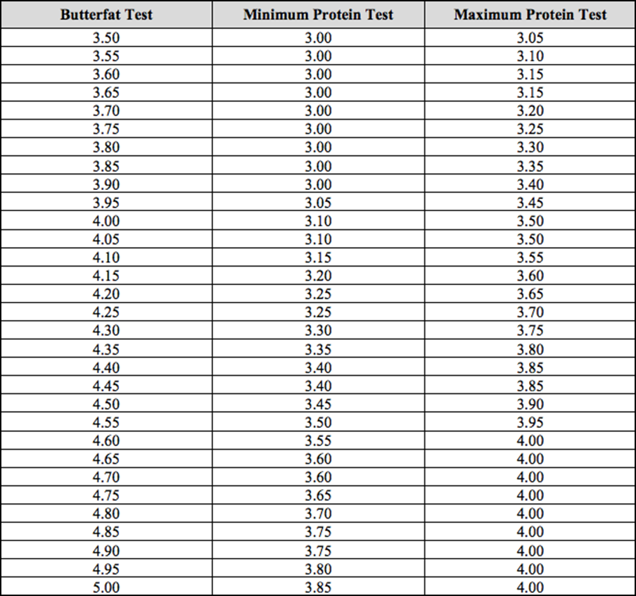
Under DRP guidelines, declared butterfat test elected can be no less than 3.50 pounds and no more than 5.00 pounds, in 0.05 pound increments. The declared protein test elected can be no less than 3 pounds and no more than 4 pounds, in 0.05 increments. Both declared components are subject to the component test ratio between butterfat and protein. The declared butterfat to protein test ratio must be no less than 1.15 and no greater than 1.30, rounded to the nearest five hundredths (0.05). The minimum-maximum component ratios are illustrated in Figure 4.

Figure 4:

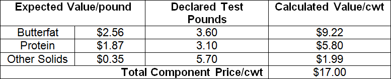
A producer using the Component Pricing option declares test values of butterfat and protein that are necessary to determine the expected total component milk price used to determine expected revenue and coverage. These producer elections using the Component Pricing option are shown in Figure 5. When determining the expected value of butterfat and protein, the average monthly value for each month in the insured quarter is calculated utilizing component futures’ prices and AMS component formulas. The total component price/cwt in Figure 5 represents an expected total component price for Q4 2019 assuming declared butterfat and protein test values of 3.60/3.10, respectively.

Figure 5:

If the component pricing option is elected, a producer’s coverage is based on their declared butterfat test and protein tests. However, to receive your full coverage, your average actual butterfat test and average actual protein test component levels for milk sold during the quarterly insurance period must not be less than 90 percent of the declared butterfat test or declared protein test.

The final butterfat test and final protein test used to calculate the final component pricing milk revenue and the actual component pricing milk revenue for indemnity calculation purposes is determined as follows:

1. If either actual component test is less than 90 percent, then, as applicable, the final butterfat test and/or final protein test will be the actual determined test value percent divided by .90. For example, if the declared butterfat test is 5.00 pounds, the policyholder’s average butterfat test during the quarter must equal or exceed 4.50 pounds. If the actual butterfat test is 3.80 pounds, the final butterfat test will be 4.22 pounds (3.80 pounds actual / 0.90).
2. For either actual component test that is at least 90 percent of the declared, then, as applicable, the final butterfat test and/or final protein test will equal the declared butterfat test or declared protein test. For example, if the declared protein test is 4.00 pounds, and the policyholder’s average actual protein test during the quarter is 3.80 pounds, the final protein test will be 4.00 pounds.

Premiums will be due in accordance with the initial component calculations; any recalculation of component values will not result in a premium refund.

Farm-Level Factors

Optional Protection Factor:

Under DRP, a producer must elect a protection factor between 1.0 and 1.5, in 5% increments. It designed to provide greater flexibility in matching farm-level production risk. For example, if a producer declares a protection factor of 1.5 and receives an indemnity payout of $20,000, their final quarterly indemnity would equal $30,000, as $30,000 = ($20,000 x 1.5). The producer’s premium increases proportionally along with any indemnity, if one is paid out. Even if there is no indemnity payout, the producer must still pay the premium times their chosen protection factor.

Yield Adjustment Factor:

Each quarter upon the release of state-level milk production data by the USDA via Milk Production reports, a yield adjustment factor will be determined for producers based on actual vs. expected production yields in their state or pooled production regions. This yield adjustment factor is determined by dividing actual quarterly milk production per cow by the expected milk production per cow for that quarter. Both the expected and actual values represent a state or pooled production region yield data, not expected or actual yield for an individual operation.

For example, if expected milk production per cow for a given quarter and state is 7,500 pounds and the USDA publishes actual milk production per cow of 7,800 pounds for that quarter and state, the yield adjustment factor would be equal to 1.04, as 1.04 = (7,800 ÷ 7,500). Similarly, if actual quarterly milk production per cow was 7,200 pounds, the yield adjustment factor would be 0.96, as 0.96 = (7,200 ÷ 7,500).

From a practical standpoint, if the yield adjustment factor is above 1.0, then actual milk revenue is calculated higher and potentially above the threshold that would trigger an indemnity payment. Conversely, if the yield adjustment factor is below 1.0, then actual milk revenue is calculated lower thus reducing the threshold for triggering an indemnity payment.

This holds true regardless of actual farm level production. In other words, the dairy’s actual production may be lower in a given quarter due to farm-level factors while the state or region’s milk production was higher than expected. It may also be true however that the dairy’s production proves larger than anticipated while the state or region’s actual production was lower than expected.

Production Loss Factor:

A dairy producer declares their covered milk production on the quarterly coverage endorsements, but if the dairy does not actually market the covered milk production that was declared by the producer:

1. If milk marketings for the quarterly insurance period are at or above 85 percent of the declared covered milk production, then your covered milk production equals your declared covered milk production, even if your milk marketings are lower than the declared covered milk production; or
2. If milk marketings during the quarterly insurance period are less than 85 percent of the declared covered milk production, then your total covered milk production for this quarterly insurance period shall equal your milk marketings divided by 85 percent.

For example, two separate quarterly coverage endorsements purchased at different points in time for a single quarterly insurance period, endorsement A has 1,500,000 pounds of declared covered milk production and endorsement B has 500,000 pounds of declared covered milk production for a total of 2,000,000 pounds. The milk marketings are 1,200,000 pounds of milk for the quarter. The total covered milk production for all quarterly coverage endorsements shall be 1,200,000 pounds divided by .85, which equals 1,411,765 pounds.

Premiums will always be due as calculated by your initial declared covered milk production, and they will not reduce because of any recalculations in covered milk production. This is important to understand as even though there is no maximum amount of milk production that can be insured, there is a disincentive to over insure since payments are ultimately determined by actual production, not declared production.

Declared Share:

A producer’s declared share, or actual share, represents the percentage interest in the insured milk as an owner of the dairy operation at the time of the quarterly coverage endorsement. The premium paid and indemnity received adjust proportionally with the declared share of a producer.

For example, if a producer owns 50% of the quarterly coverage endorsement under the DRP program, they only have to pay 50% of any premium costs, but will only receive 50% of any indemnity payouts.

DRP Frequently Asked Questions (FAQs):

The USDA Risk Management Agency (RMA) has released a FAQ sheet to answer any additional questions that individual producers may have regarding Dairy Revenue Protection, which can be found online at:

https://www.rma.usda.gov/help/faq/dairyrevenueprotection.html

Conclusion

Dairy Revenue Protection represents a new opportunity for producers to address the very realistic risk of a significant and unexpected decline of future revenues and overall profitability. CIH embraces any new tool that offers the dairy industry an ability to protect against declining milk revenues and enhance overall profitability. Protecting revenue at a government-subsidized rate is especially attractive in low margin environments, particularly when premium costs are not due until the end of the period being covered. It is critical to assess how farm-level factors and features under DRP relate to your specific operation. CIH will work alongside your operation to create an integrated margin management policy that ensures you are properly hedged and able to take advantage of greater revenue opportunities if offered above the minimum level of your DRP. We encourage you to learn how a combination of risk management strategies can help you protect and enhance forward revenues and, ultimately, overall profit margins for your dairy operation.

For any questions or to learn how this may specifically affect your dairy, contact CIH at 866-299-9333.

With hog margins currently at some of the most depressed levels in years, many producers are understandably concerned with the price they are receiving for their pigs. While much of the present situation is beyond the producer’s control, such as tariffs and trade issues, there are other areas where they can exert more influence. Controlling costs is certainly one of those, and many operations have already made adjustments to become more efficient. Another area that may be one to look at is how they are paid by the packer for their pigs. Most producers deliver hogs off formula contracts, where the pricing mechanism is determined in advance and remains consistent over the life of the contract. These may include some differential from the CME Lean Hog Index for example, or be a function of some cash price as reported by USDA such as a percentage of cutout or differential from Western Corn Belt.

Considering a New Contract?

Many producers reading this may already be considering a new packer contract or in the process of renegotiating their current packer agreement. With the new plants that have recently opened, some producers have been approached by packers looking for pigs to fill their schedules and offered contracts with pricing features that differ from those they are currently using. You may be curious about how these contracts would have compared historically with how you are presently being paid for your pigs. Also, to the extent that a new packer or your existing packer may be presenting new offerings to choose from, you may wonder whether you would be better off with one alternative over another.

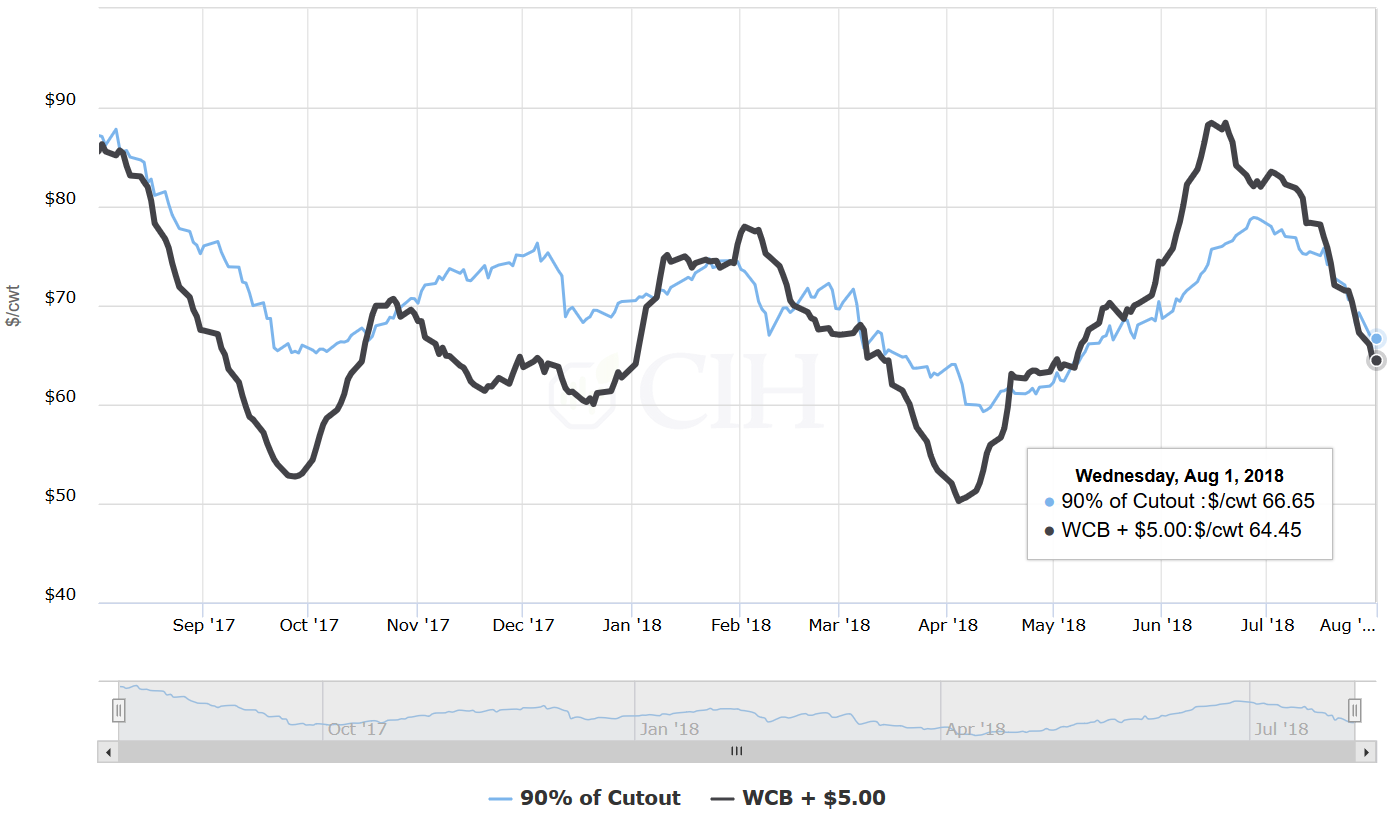
Fortunately, there is a way you can make these comparisons and analyze various contract alternatives to help inform decisions about how to negotiate with a new packer or renegotiate with your existing packer. As an example, you might compare two different offerings to see how they would have stacked up against each other in past years. In addition to providing a historical price comparison, this would also allow you to measure basis variance between the two in order to help gauge whether one contract may have been more favorable than another. We can look at a specific example comparing the difference between 90% of cutout for instance against the Western Corn Belt plus $5.00 to see how these two payment formulas would have differed historically over the past five years.

Figure 1 shows the comparison of these two price series over the past year. You will notice that the contract based off 90% of cutout is currently higher than the WCB plus $5.00 contract by $2.20/cwt. ($66.65 versus $64.45). As a result, it would be more favorable to deliver pigs in the spot market against the contract priced off of the cutout rather than the WCB contract. You may also notice though in the comparison of the two price series that up until quite recently, it was actually much more favorable to be priced off of the WCB contract compared to the cutout formula, in some cases by almost $13/cwt.

There were other times however, such as earlier this spring and particularly last fall, when it was significantly better to have been priced off the cutout contract relative to the WCB formula. In addition, you can see that there has been more variance in the past year with the WCB contract price series than the cutout contract series. While both were priced very closely together at around $88 last summer, the lows in the WCB plus $5.00 series show much deeper troughs while conversely, the recent high has also been much more of a premium as compared to the 90% of cutout series.

Figure 1. 90% of Cutout Versus WCB + $5.00

We can also look at the historical variance of the two price series by comparing both price and basis in the following table of Figure 2. This comparison measures current values against averages over the past 1, 3 and 5 years of history. Here again, we can see that being priced off 90% of cutout is currently more favorable than having a contract based on WCB + $5.00, with both the 1 and 3 year averages showing the cutout contract to likewise be superior. However, a longer term view taking a 5-year average shows the price of WCB +$5.00 to be slightly higher by about $0.60/cwt.

Figure 2. 90% of Cutout Versus WCB + $5.00

These comparisons can also be shown visually in graphs with some interesting observations. Note that the previous chart comparing the past year of price performance indicated more variance in the WCB price series versus that of the cutout series. While this has been true over the past year, the basis history reveals something different. Figures 3 and 4 show the five-year basis ranges for both the WCB + $5.00 versus 90% of cutout, respectively. In both cases, the CME May Lean Hog futures contract has been excluded from the basis calculations. You will notice that the range of basis for the WCB + $5.00 price series has been $29.51/cwt. over the past five years, with a maximum value of $13.22/cwt. positive to $16.29/cwt. negative. Conversely, the range of basis for the 90% of cutout series has been wider at $44.52/cwt. during the same time interval, with a maximum value of $24.41/cwt. positive to $20.11/cwt. negative. It may be misleading therefore to conclude that you would be assuming more risk with the contract based off the WCB + $5.00, despite the relative price performance of each during the past year.

Figure 3. WCB + $5.00 Five Year Basis Range

Figure 4. 90% of Cutout Five Year Basis Range

Another useful feature of being able to compare contracts side by side is to help with anticipating kill checks upon delivery. In addition, a producer may have more than one type of contract with the same or different packers. To the extent that the producer has some flexibility with their delivery schedule, they may find it advantageous to channel their deliveries to maximize the value of their hogs in the spot market. As an example, a producer with existing contracts priced off the comparison in this example would have an incentive to market as many hogs as possible right now against the cutout contract before delivering against the WCB contract. This could add incremental value to their marketings by maximizing the basis differential between the two pricing mechanisms.

It should be noted that the comparisons used in this example are presented for illustration purposes only, and are not meant to replicate any specific packer contract offerings. These examples are also not being presented to endorse one type of pricing mechanism over another. You should understand the exact features of any packer offering before making specific comparisons between contracts in order to draw your own conclusions on which type of contract may be a good fit for your particular operation.

For more information on how these studies were created or for help understanding how to navigate packer contracts, please feel free to contact us directly. While much of the current hog margin landscape is beyond control, there are things that producers have more sway over. The ability to better understand and negotiate packer contract offerings is definitely something a producer can leverage to help increase revenue and mitigate losses in the present environment, and there are tools to help them in this process.

National Agricultural Statistics Service (NASS) is responsible for the task of providing production and yield estimates for most crops grown in the United States. As the growing season progresses for each crop grown domestically, NASS provides their projections to the United States Department of Agriculture (USDA).

The USDA in turn will incorporate the projections into the monthly report of World Agriculture Supply and Demand Estimates (WASDE). Like making sausage, much goes into the process of yield and production projections, and in truth, we may or may not want all the details, but here we will try to explore in general how NASS makes the sausage, with a focus on corn and soybeans.

Before any yield or production projections are possible, NASS first collects data on acreage. Two surveys suit this purpose. One in March, and the other in June. Both query farm operations during the first two weeks of each month, the former on intentions, and the latter on actual plantings. For instance, last March NASS sampled approximately 82,900 farmers on what and how much of a crop they intended to plant come spring. The 2018 Prospective Plantings report revealed intentions of 89.0 million acres of soybeans and 88.0 million acres of corn seedings. The second survey, just released in late June’s Acreage report, honed in the estimate with actual plantings of 89.1 million acres of corn, and 89.6 million acres of beans, using similar survey methods.

The June Acreage is critical for NASS going forward, as it forms the basis for their estimate of harvested acres of each crop, which obviously is crucial in determining a production projection. NASS monitors the planted acreage estimate throughout the growing season, and usually only makes adjustments because of weather related anomalies. If this is the case, NASS may re-survey and revise the planted and harvested acres projections in the August Crop Production report. This occurred in 2015 when NASS re-surveyed soybean producers in Arkansas, Kansas and Missouri, as excessive wetness affected the crop and resulted in a reduction of 800,000 planted and 900,000 harvested bean acres.

In August, NASS’ survey derived yield forecasts step into the limelight, and replace a weather adjusted trend line yield based econometric model. The model relies on data from the 1988-2017 period, and projects yields on the initial new crop balance sheets in May, as well as the subsequent June and July WASDE reports. June and July WASDE yield projections will be adjusted from initial May estimates in years that experience extreme weather deviations, hence weather adjusted model. The USDA references the exact model for yields in the report footnotes.

Prior to the August WASDE report, NASS conducts dual surveys beginning in late July each new crop year, and repeats the surveys each month through harvest. The Agricultural Yield Survey (AYS) draws from farmers who responded to the planted acreage survey conducted in June, up to 27,000 operations. NASS queries the selected producers to confirm the amount of the crop seeded, and provide a best forecast of final yield based on their history and experience each month. The other survey, the Objective Yield Survey (OYS), takes actual plant counts and measurements, from plots again selected from respondents of the June acreage survey. This sample size is much smaller, roughly a quarter of the AYS, as it is more costly to administer, and draws only from a cross section of the largest corn and bean producing states. The purpose of the OYS is to smooth out the inherent subjectivity of the AYS.

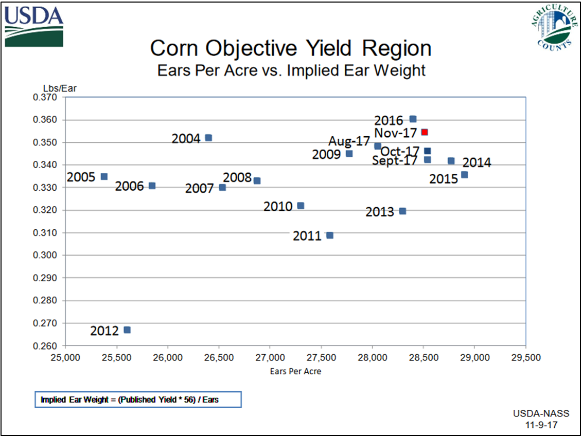
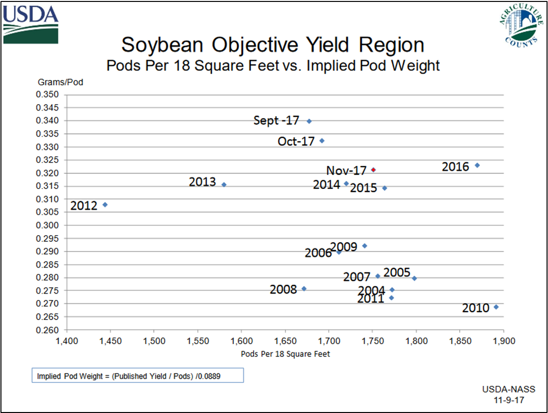
For the annual study, NASS chooses sample plots of corn from the ten largest producing states, and bean plots from the top eleven. Professional statisticians from each of these states train field enumerators in the desired methods of reliable field data collection. Depending whether it is late July or November, or sometime between, the enumerators count, measure or record specific categories of data each month. Corn data largely focuses on number of ears per acre and implied ear weights, while bean data looks mainly at pod counts and implied weights. The information gathered from the field plots is then distilled and published in charts like the examples below, taken from 2017 crop reports.

Up until now, we have described in the most basic and general terms how NASS conducts the dual yield surveys, but how do they combine the two into that savory sausage of yield forecasts? The likes of which may set off choruses of debate each year between agricultural producers, analysts and market participants alike, generating screams of where did that number come from? Think August 2017, WASDE corn yield estimates of 169.5 bpa, well above expectations as drought conditions in the High Plains and throughout parts of Iowa, had all braced for worst-case scenarios. Enter the NASS designated Agricultural Statistics Board (ASB), who take the data from both surveys and are charged with arbitrating the subjective nature of the AYS and the empirical evidence from the OYS to arrive at their best estimate of corn and soybean yield projections for each monthly report, again beginning in August. The total production estimates are a factor of the previously gathered acreage projections and the up-to-date yield approximations. While the production formula is clear, the yield forecast is the sausage with secret ingredients that only the ASB knows.

As the calendar turns, and harvest approaches, it makes sense that the job of the ASB perhaps becomes a bit less complicated, as they are dealing with more certainty as each day passes. The farmers’ AYS becomes more certain as crop maturity nears, no more best estimation of final yields based on history and experience, but rather producers can see how it actually looks. The OYS also has the benefit of actual ears and pods to count and weigh as time moves forward, rather than an implied measure of the two.

With the recent release of the Acreage report, the agricultural markets await the all-important August WASDE report, where the dual NASS surveys of farmers and field studies mash up to give indications of corn and bean yields. Let the debates begin!

References

Irwin, S., and D. Good. “Opening Up the Box: More on the USDA Corn Yield Forecasting Methodology.” Farmdoc Daily (6):162, Department of Agricultural and Consumer Economics, University of Illinois at Urbana-Champaign, August 26, 2016.

The Yield Forecasting and Estimating Program of NASS, by the Statistical Methods Branch, Statistics Division, Nation Agricultural Statistics Service, U.S. Department of Agriculture, Washington D.C., April 2012. NASS Staff Report No. SMB 12-01.

Understanding Crop Statistics. Frederic A. Vogel, National Agricultural Statistics Service, and Gerald A. Bange, World Agricultural Outlook Board, Office of Chief Economist, U.S. Department of Agriculture. Miscellaneous Publication No. 1554.

One of the main economic functions of the futures market is price discovery. Participants from all over the world place bids and make offers in a dynamic auction to determine the value of a commodity or financial instrument at any given point in time. Because multiple contracts trade simultaneously for the same commodity in different time periods, both nearby as well as in deferred months and years, this price discovery process is multi-dimensional. It not only reveals the current or “spot” value but also expectations about how that value will change over time. Studying this relationship, referred to as the forward curve, can provide valuable information on how market participants anticipate future price movements for the cash market. It also can help hedgers refine position structure to protect risk in deferred time periods.

The Cash and Futures Relationship

Futures contracts are called derivatives because they derive their value from the underlying cash market. Based on the contract specifications, futures either settle to the cash market through physical delivery as is the case with contracts like corn, or are cash settled where their final value at expiration is determined by some sort of an index as is the case with hogs. In either case, prior to a contract’s expiration and convergence with the cash market, there is a difference in value between the spot cash price and the nearby futures price. This difference, or basis, changes over time where in some cases the cash price may be at a premium to futures, and in others a discount.

Looking beyond the nearby futures contract, deferred futures also may be trading at premiums or discounts to the cash market as well as to nearby futures. One of the reasons why deferred futures prices may trade at a premium to spot prices could be seasonality. For many commodities, there is a normal tendency for prices at certain times of the year to be higher or lower than other times of the year, and the futures curve reflects those seasonal tendencies. Another reason may be fundamental. As an example, there may be a shortage of the commodity in the spot market although the pipeline might suggest ample supply in a deferred period. In such a case, the spot or cash price would be trading at a premium to forward futures prices.
The Hog Market

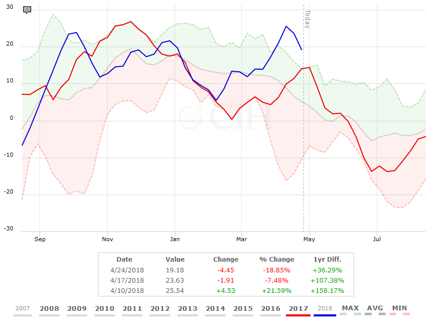
The current structure of the hog market offers one example of the relationship between cash prices and the forward futures curve. Notwithstanding a recent recovery, the cash hog market has been under heavy pressure since late January as supplies have been larger than expected. After starting the year at prices very close to the average of the past 10 years, the CME Lean Hog index declined almost $22/cwt. between late January and early April as hog slaughter and pork production have posted strong year over year increases from 2017 (see Figure 1). Total hog slaughter during Q1 was 31.075 million head, up 3% from a year ago; however, pork production of 6.645 billion pounds during the quarter was 3.7% higher than last year as hogs are coming to market at heavier weights.

Moreover, the latest USDA Hogs and Pigs report indicated that supply growth is likely to continue through the summer and into fall. The hog breeding herd on March 1 was estimated at 6.2 million head, the largest since 2008 with producers reporting that they intend to farrow more sows than a year ago for the next two quarters. March-May farrowing intentions were up 2.1% from 2017 while the June-August quarter showed an increase of 1.4% from last year. Recent news of China’s decision to impose retaliatory tariffs on U.S. pork imports hasn’t been helpful either as much of the offal goes to that market with limited opportunities for other outlets.

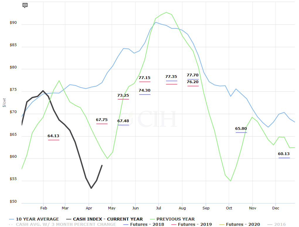
Looking at Figure 1, you will notice that the loss in value in the CME Cash Hog Index and subsequent recovery was very similar to last year (green line) albeit around 3 weeks early in 2018. You will also notice the hash marks spread across the page, which represent futures prices as of April 26. The blue lines correspond to 2018 futures while the red lines are the values for futures in 2019. Each value is displayed in the middle of the month when the futures contract expires. The 67.48 value in blue between the month of May and June represents the current value of May 2018 futures which is where the black line is headed over the next few weeks. Given the two values have to converge at expiration, this means that either the black line (spot cash market) needs to rise further, and/or the price of May futures needs to come down in order for the two to converge by mid-May.
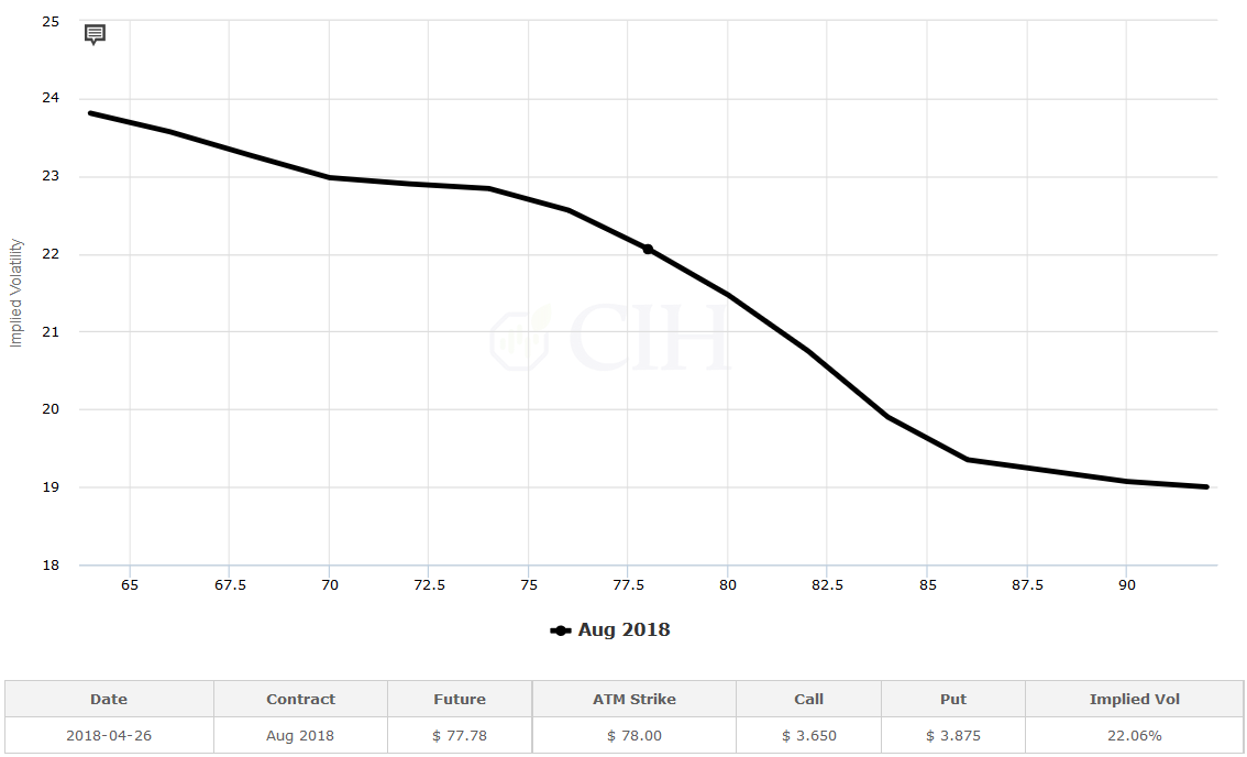
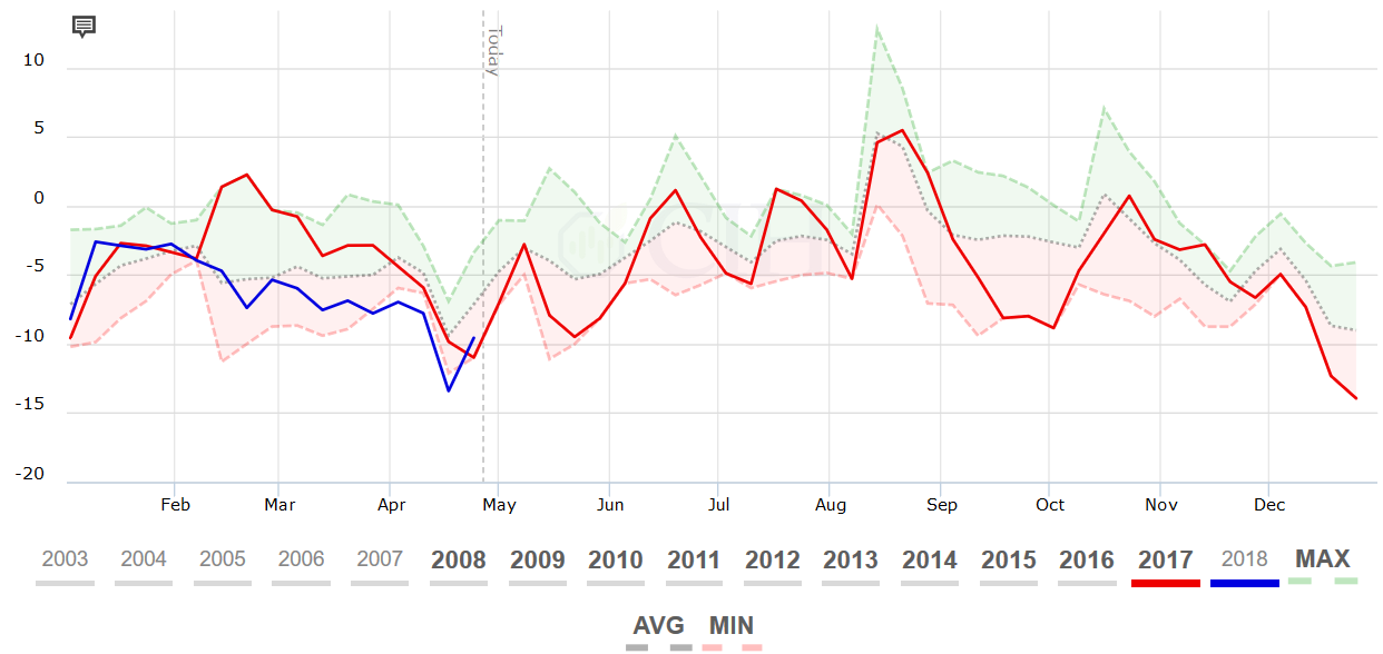
The summer futures prices with June at 74.30, July at 77.35, and August at 77.70 indicate expectations for a continued rise in the cash market or CME Lean Hog Index over the next few months as would seasonally be expected, although those expectations are much more muted than the increase in cash prices we witnessed last year when looking at the green line. This likely is due to the factors previously mentioned with larger hog slaughter and pork production relative to last year and increased trade uncertainties. From a hedging perspective, while the futures market represents a fair estimate of value for summer hogs based on what is currently known, it may make sense for a producer to retain upside flexibility on their price hedges in case the cash hog market is stronger over the next few months. As a counterpoint however, it should be noted that August Lean Hog futures are also currently trading at their highest premium relative to the CME Lean Hog Index in the past decade (see Figure 2).

An example of how a producer might address both of these considerations in a hedge would be adding long call options to a short futures hedge or cash sale in the local market against their summer marketings. The August futures are trading around 77.70, so the producer might purchase a call option with an $80 or $82 strike price to address the opportunity cost in a higher market against pre-existing sales either in the cash market or on the board. They may even choose to offset part of the cost of purchasing the call by selling put options below the market. This not only would lower the cost of adding upside flexibility to the hedge, but also take advantage of the current option volatility skew in the market as higher strike calls are trading at lower implied volatilities relative to lower strike puts (see Figure 3).

Another consideration for a hog producer from a hedging perspective concerns cash basis levels. With the cash market trading at a discount to futures, hog basis is currently negative and has actually been running at or near new 10-year lows through the month of April (see Figure 4). Because of this, a producer would only want to deliver hogs against the minimum amount necessary to meet packer commitments, and possibly even slow down hedge removals against their marketing schedule.

The Cattle Market
By contrast, the forward curve in cattle offers a different perspective on the relationship between cash and futures prices as well as the implication for hedgers. Unlike the hog market where cash prices are currently trading at a discount to futures, spot cattle prices in the cash market are at a premium to the forward curve. Despite the fact that the number of cattle on feed as a percentage of the previous year has consistently run 107%-109% over the past several months, much of the cattle placed into feedlots last fall were lighter weight animals that require more days on feed to reach market weight. As a result, cattle marketings and slaughter have not kept up with demand as packers have large commitments they need to fill in the spot market.
Because of the heavier placements over the past several months however, expectations are that an abundant supply of cattle will be available to the market during the summer marketing period. Since market participants anticipate this increased supply of cattle and beef production over the next several months, the forward curve reflects these expectations with lower prices for summer contracts relative to the spot spring period. Prices are gradually expected to increase heading into the fall and winter from a summer low against the June and August contracts. Figure 5 shows the forward cattle curve out through August, 2019:

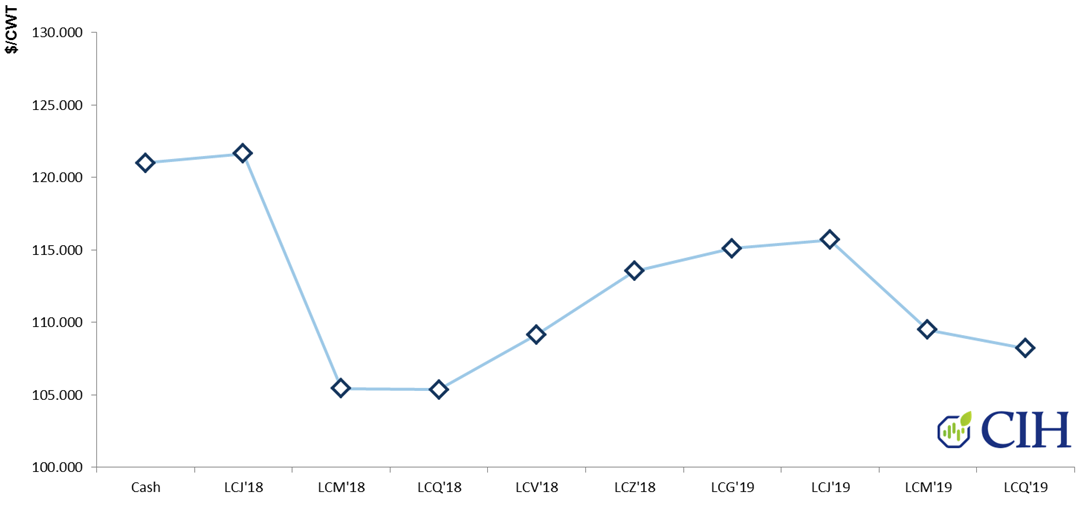
Compared to the hog market, the relationship between cash cattle and forward futures implies a much different scenario for cattle producers in managing their inventory and hedge positions. Unlike hogs, the basis has been strong for cattle. Figure 6 displays the current cash basis for live cattle in the Texas, Oklahoma, and New Mexico region, which has been running at or near 10-year highs over the past month. The historically strong cash basis which is well above average provides a strong incentive for producers to market early and pull supplies forward, hopefully alleviating the possibility of excess supply later in the summer.

Meanwhile, because the forward curve is discounted relative to spot futures and the cash market, a cattle feeder would also be encouraged to maintain upside flexibility in their hedges against summer marketings. Similar to hogs, a cattle feeder might likewise consider adding long call options to a short futures position. Alternatively, they may choose to protect downside price risk on their physical inventory by simply purchasing put options. Depending on their projected breakeven levels, they could finance the purchase of puts by selling upside calls to establish a maximum price on a portion of their inventory.

The Corn Market
Another example of the relationship between the cash market and the forward futures curve is the corn market. After harvesting another bumper crop last fall on record yields that maintained corn stocks at historically high levels, cash corn prices have been depressed with limited expectations for much of a recovery. Recent drought conditions in Argentina however and lower than expected intended acreage revealed in USDA’s Prospective Plantings report has put some risk premium back into the market. In addition, cold and wet weather which has extended through April across much of the Northern Corn Belt has delayed planting progress and likewise added a risk premium to the futures market.

Unlike hogs or cattle, corn is a storable commodity and the relationship between prices of futures contracts on the forward curve typically reflects a “cost of carry” or storage between delivery months. In a situation like the present where supplies are plentiful, there will be a positive carry such that deferred futures are trading at a premium to nearby futures, reflecting the cost of storing the crop between expirations. In a case where there is a shortage, such as in a drought like the 2012-13 crop year, there will be a negative carry or a premium on nearby futures relative to deferred futures contracts. This provides a disincentive for producers to hold on to their crop as they effectively lose money storing between expirations. Figure 7 displays the current forward curve for corn:

For a corn producer, the forward curve on corn implies different considerations for managing hedge positions between old-crop corn in the bin and new-crop corn which is now being planted. Looking at the first half of the curve representing the 2017-18 old-crop marketing year, there is a positive carry as previously mentioned. In other words, the producer is incentivized to hold on to their crop in order to capture the carry in the market. Assuming the producer has storage, they therefore would want to maintain a short hedge in the deferred July or even September futures contract against their physical inventory, representing the horizon of the old-crop price curve.
Another way of looking at this would be to analyze the spread between old-crop and new-crop corn within a historical context. Figure 8 shows the spread between the spot May Corn futures contract and the new-crop December futures contract. You will notice that the 25-cent discount of May relative to December is the same as last year and near a 10-year low for this time of year.

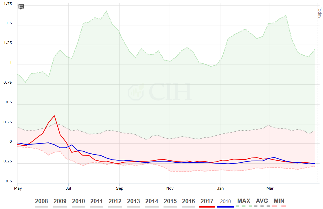
Looking out to new-crop however, the forward curve is telling us something different. Given the previously mentioned dynamics of lower intended acreage and delayed planting progress that has been compounded by the crop losses in Argentina, the second half of the forward curve starting with the new-crop December contract is relatively flat. This is because a majority of the open interest or price discovery in new-crop corn is in the December futures contract, which has been bid relative to the forward contracts on the curve. While the March, May, and July 2019 futures contracts are trading at successive premiums to December 2018 futures, these premiums are relatively small from a historical perspective.

If we look at a similar chart to Figure 8 which now compares the December 2018 futures price relative to the July 2019 futures price, you will notice in Figure 9 that the 16 cent discount of December futures relative to July for new-crop corn is at a 10-year high for this point in the season. As a result, unlike in old-crop where a corn producer would be incentivized to place their short hedge as far out as possible on the curve; in new-crop, there is an incentive to keep the short hedge on the front end of the curve in the December contract, and wait for more carry to be built into new-crop spreads.

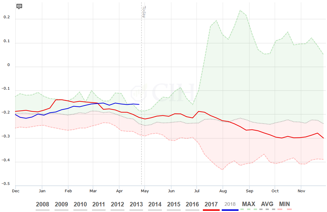
The forward curve is an important component of the price discovery process in the futures market and provides valuable information for a risk manager to consider when evaluating their exposure. Understanding the relationship between cash and futures can help producers better manage their hedge positions and leverage the information being provided by the market to take advantage of opportunities that may present themselves.

There is a risk of loss in futures trading. Past performance is not indicative of future results.

The Commodity Futures Trading Commission (CFTC) publishes a weekly report which breaks down the total open interest as of each Tuesday’s settlement for markets in which 20 or more traders hold positions equal to or above reporting thresholds established by the Commission. The reports are released every Friday and provide market participants insight on how open interest is distributed among different groups of traders. In a very general sense, it breaks open interest down into two categories – reportable versus non-reportable positions – but other classifications have been distinguished by the CFTC to provide further insight on the participation of different type of traders in the market.

History and Breakdown of the Reports
Antecedents of the Commitments of Traders (COT) reports can be traced all the way back to 1924 when the USDA’s Grain Futures Administration, the predecessor to the USDA’s Commodity Exchange Authority and later the CFTC, published its first comprehensive annual report of hedging and speculation in regulated futures markets. Beginning in 1962, the reports were published monthly followed by a mid-month and month-end version in 1990, then every two weeks in 1992, and finally a weekly format in 2000. The data is also now compiled and released on a more timely basis, and has since moved from a fee-based subscription to becoming freely available on the CFTC’s website at the following link: https://www.cftc.gov/MarketReports/CommitmentsofTraders/index.htm

The CFTC collects position data from reporting firms including clearing members, futures commission merchants (FCM’S), foreign brokers and exchanges. While the position data is collected by these various reporting firms, the actual category or classification of traders’ predominant business purpose is self-reported by the individual traders on the CFTC’s Form 40 which is reviewed by commission staff for reasonableness and accuracy. Traders are able to report business purpose by commodity, and therefore may be classified differently for one market versus another.

There are four reports, including legacy, supplemental, disaggregated, and traders in financial futures. The legacy reports are broken down by exchange and include a futures only and a combined futures and options report. Legacy reports break down the open interest into two categories – non-commercial and commercial traders. Supplemental reports break down the reportable open interest into three trader classifications: non-commercial, commercial and index traders. The index trader classification was added in 2007 to provide the marketplace with more transparency on positions in exchange-traded markets, with further classifications subsequently added with the disaggregated report in 2009.

The disaggregated report increased transparency by separating traders into the following four reportable categories: Producer/Merchant/Processor/User, Swap Dealers, Managed Money, and Other Reportable. This development evolved from confusion over what types of traders were holding various positions in the markets. Generally speaking, the legacy form of the report which only defines two categories of traders as commercial or non-commercial were historically seen as hedgers and speculators, respectively. Traditionally, these participants were viewed as those whose positions were tied directly to the physical commodity versus those who had a purely financial interest in the market.

It became clear over time however that there was a need for further distinction. Commodity index fund trading which grew substantially in the early part of the century brought about the initial need for added transparency as these entities held long-only positions in the futures market to replicate holding commodities as an asset class. With large reportable positions, they defined themselves as commercial traders given that their trading was considered a hedge against the underperformance of the various portfolio benchmarks as defined in their fund prospectuses.

The rise of swaps in the commodities market likewise provided another catalyst to further clarify the breakdown of open interest in the commodity markets. Financial entities including FCM’s and other market participants have increasingly been offering structured products to clients that mimic or are backed by exchange-traded futures and options. Here too, the purpose of trading for these entities was to hedge the financial commitments they had with their counterparties in a swap agreement, and it became necessary to define this category separately from commercial traders.

Report Data
The CFTC provides the Commitments of Traders data in both a long and short format. The short format displays open interest separately by reportable and non-reportable positions. For reportable positions, additional data is provided for commercial and non-commercial holdings. This shows total long positions, total short positions, spreading positions, changes from the previous report, percent of open interest by category, and numbers of traders by category.

“Spreading” is a computed amount equal to offsetting futures in different calendar months or offsetting futures and options in the same or different calendar months. Any residual long or short position is reported in the long or short column. Inter-market spreads are not considered. The following table shows an example of the short format for the legacy version of the report for CBOT Corn futures and options combined:

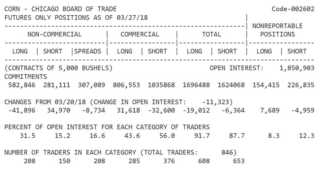
The long version of the report also groups the data by crop year, where appropriate as in the case of corn, and shows the concentration of positions held by the largest four and eight traders. The supplemental report is published for futures and options combined in selected agricultural markets and in addition to all of the information in the short format, also shows the positions of index traders. The non-commercial and commercial positions are typically viewed without the impact of the index trader category to analyze changes in positions over time. The reason for this will be explained in the examples to follow under the analyzing the data section.

The disaggregated report evolved from a recommendation to the Commission in September, 2008 to remove or disaggregate swap dealers from the commercial category and create a new swap dealer classification for reporting purposes. In addition, a “money manager” category was also created which for the purpose of this report is a registered commodity trading advisor (CTA); a registered commodity pool operator (CPO); or an unregistered fund identified by the CFTC. These traders are engaged in managing and conducting organized futures trading on behalf of clients. Every other reportable trader that is not identified as a producer/merchant/processor/user, a swap dealer, or a money manager is thus classified in the “other reportables” category. The following table shows an example of the short format for the disaggregated version of the report for CBOT Corn futures and options combined:

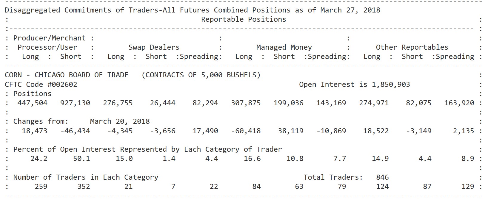
Analyzing the Data
Traders often look at data in the COT reports for clues on market direction and use it as an indicator of potential changes in price trends. Just as with any indicator, there are limitations to using the data as a technical trading tool; however, careful scrutiny of the reports can provide valuable insight when used in conjunction with other market resources. As an example, let’s analyze the recent activity in the corn market. Going back to the basics of the data in the legacy reports, there are two main classification of traders – commercial and non-commercial. The commercial trader touches the physical commodity and their positions are hedging against the risk of an adverse change in value on the physical ownership. This group is therefore always net short the market as they are holding positions against long physical in the cash market. The following chart shows 10 years of history for the net commercial corn position:

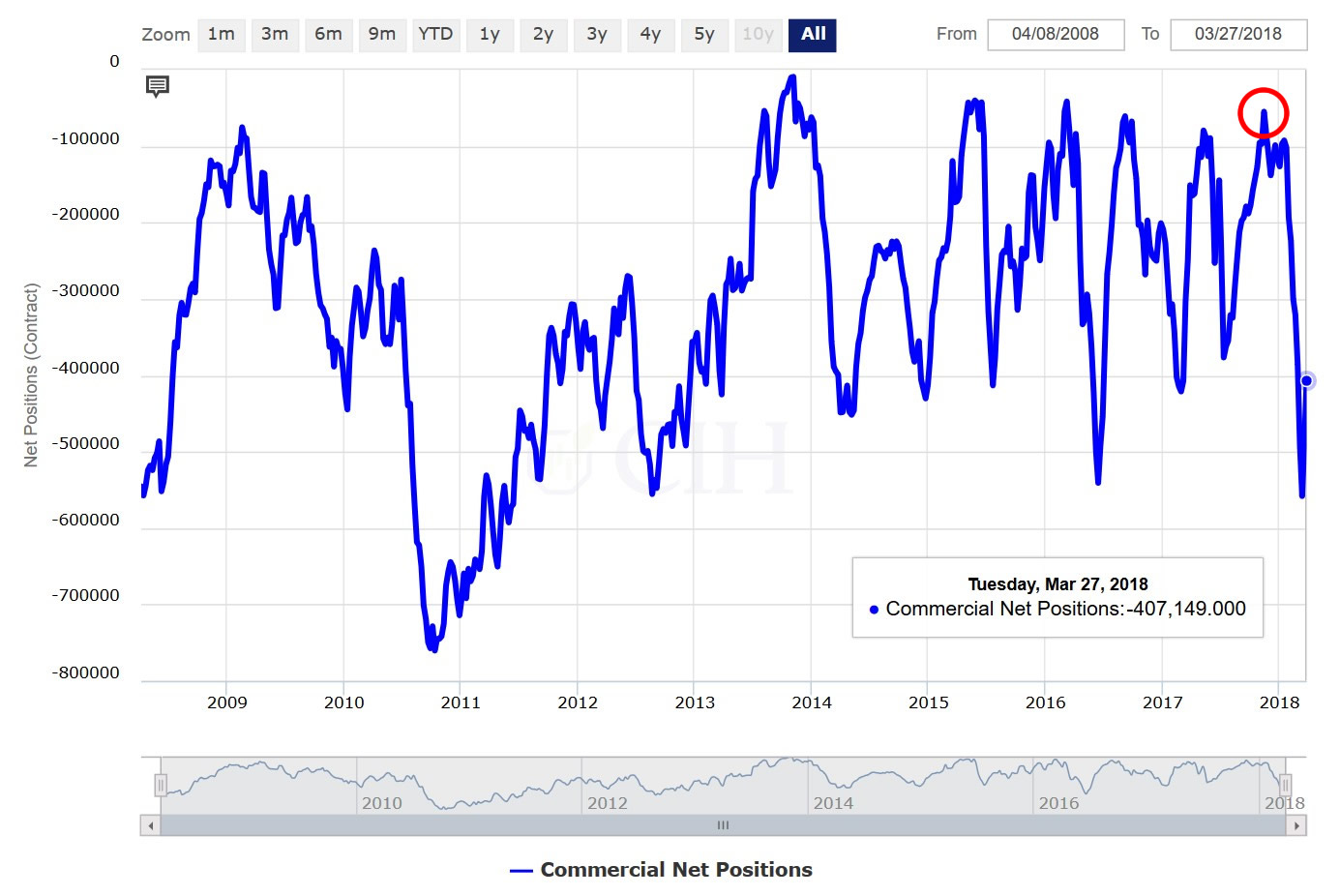
Conversely, the non-commercial trader does not touch the physical commodity and is not hedging risk of adverse price movement in the cash market, although this collective group of traders may be either net long or net short the market depending on their price bias and market outlook. While the legacy report historically has not considered the impact of index traders on this category of open interest, it is possible to separate out the Commodity Index Trader position when analyzing the data based on the supplemental report that has been in use for over 10 years now. Because the CIT position is always net long (see chart below), this provides us with a more accurate view of the non-commercial net position.

Since the CIT is mostly a passive, long-only market participant, if we look at the non-commercial net position without this component, we get a better picture of the speculative participation in the market:

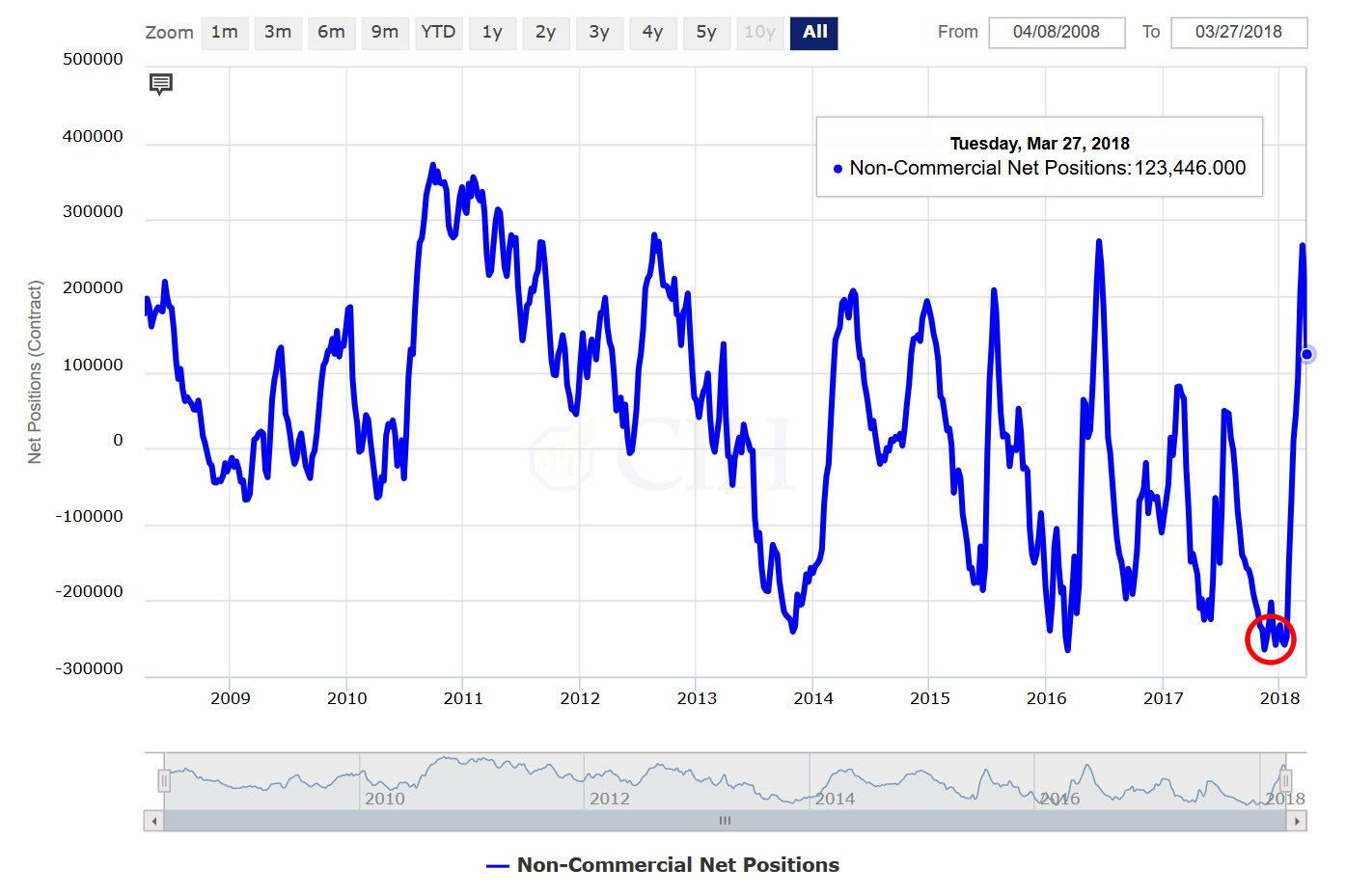
Notice in the commercial and non-commercial charts above, there are two highlighted areas of interest represented by the red circles. Each of them corresponds to a roughly two-month period between mid-November and mid-January when there was a historical divergence between the two data series. The net commercial short position was nearly the smallest of the previous 10 years at the same time that the net non-commercial short position was the largest. This divergence between the positions of the two main categories of open interest also was occurring in conjunction with corn futures that were trading at the bottom decile of the previous 10 years of price. Another interesting point to note about the corn market during this period was that the divergence in the COT data was also developing at a time when there historically is a tendency for prices to be at a seasonal low:

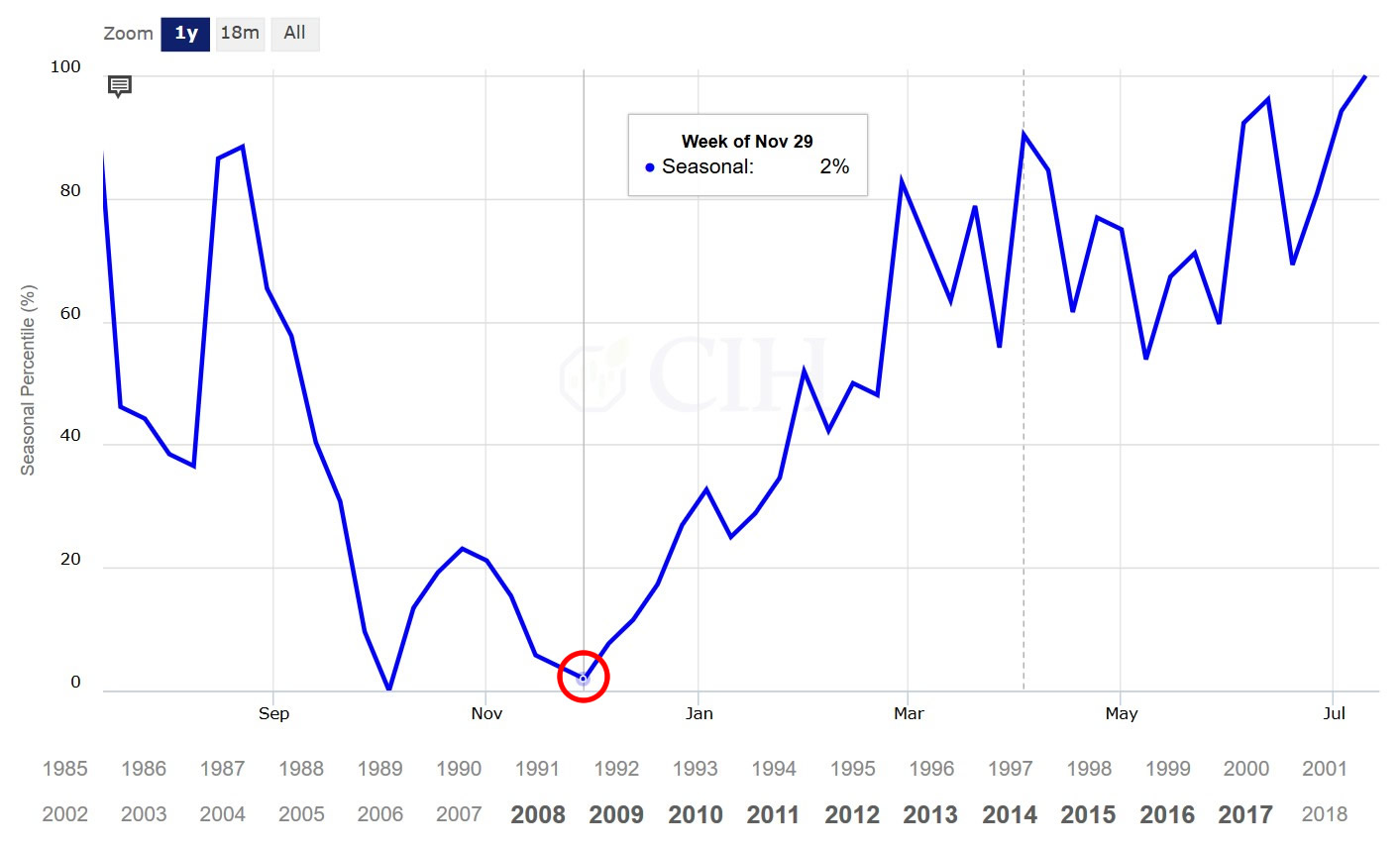
While not necessarily a bullish signal in and of itself, the divergence in the COT data late last year did provide a warning sign for a corn market that had been trending down for months and was mired in deep bearish sentiment. With speculative short interest already at a historical extreme, it suggested that there were very few if any incremental sellers left to continue pressuring the market lower. This can also be seen looking at a price chart of corn from that time as the momentum of the downtrend had slowed substantially during Q4:

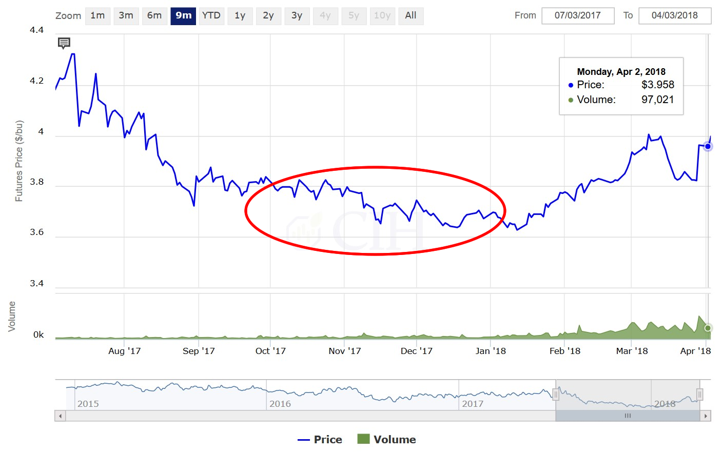
Moreover, if there were some catalyst to begin moving prices higher, as the drought in Argentina subsequently provided, speculative short-covering can quickly fuel an unexpected price advance. While the corn market represents an obvious example with the divergence between commercial and non-commercial net positions at historical extremes, sometimes hints in the CFTC COT data are more subtle. The recent hog market is a good case in point as an example of a bearish divergence. Although the absolute value of the net commercial short position and the net non-commercial long position were not at historical extremes, they were showing a pretty stark divergence seasonally for that time of year based on 10 years of data for early January:

Unlike the corn market example, where prices historically were trading at extreme levels with a seasonal tendency to move in the other direction, the hog market was beginning to flash other warning signs such as weekly slaughter running well ahead of what was implied by the December Hogs and Pigs report. Spot April Lean Hog futures prices have since dropped around $20/cwt. from the highs back in early January:

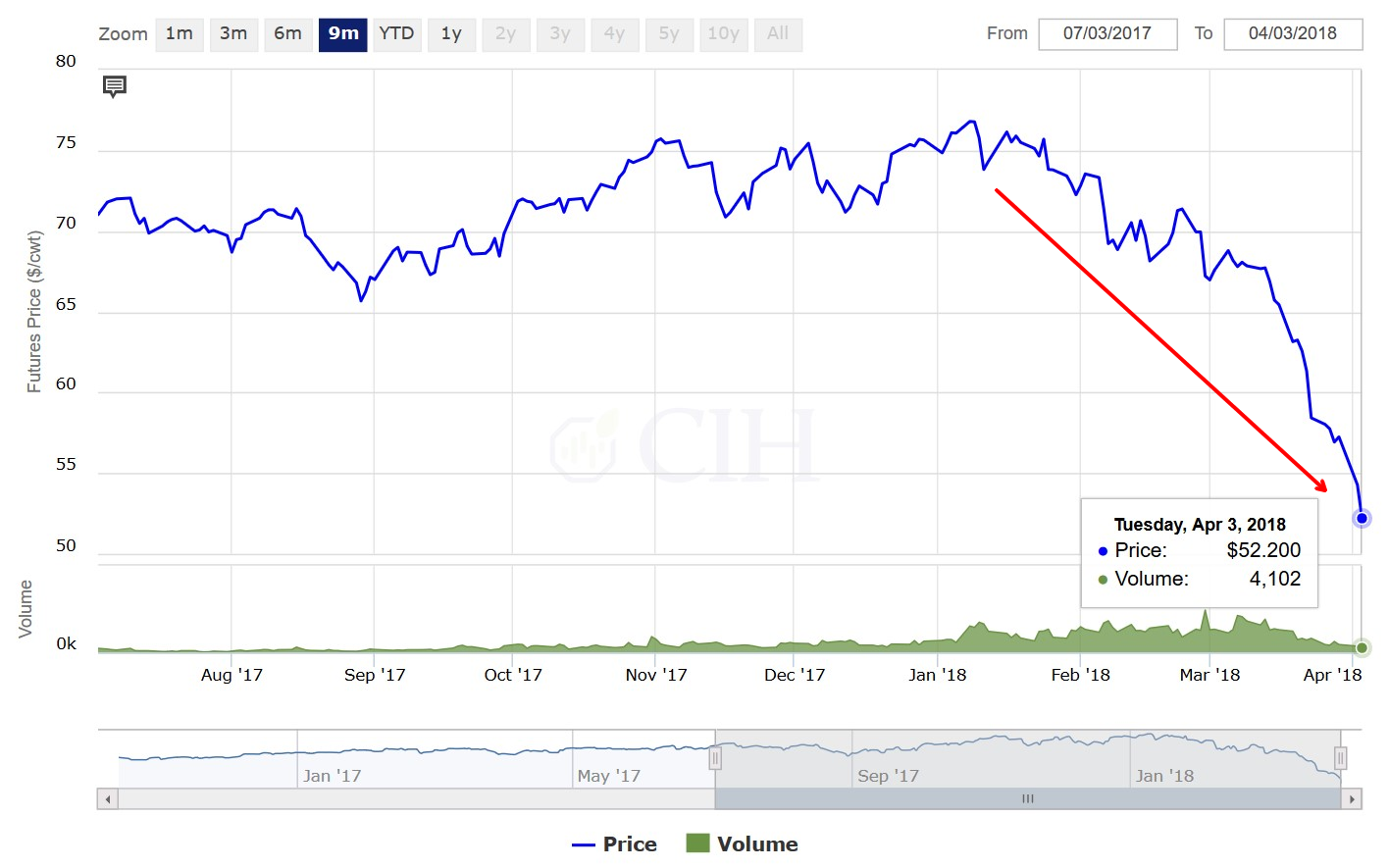
Although the CFTC Commitments of Traders data by itself does not provide a definitive signal for price direction in any particular market, it nonetheless has value in shedding light on the breakdown of open interest and how positions are distributed across the various participants in the market. It is definitely a resource that should be understood, evaluated, and considered as part of a trader’s decision to initiate and manage positions in the market.